Contents
Scroll to:
https://doi.org/10.23947/2687-1653-2021-21-4-346-363
Scroll to:
The use of data mining and machine learning tools is becoming increasingly common. Their usefulness is mainly noticeable in the case of large datasets, when information to be found or new relationships are extracted from information noise. The development of these tools means that datasets with much fewer records are being explored, usually associated with specific phenomena. This specificity most often causes the impossibility of increasing the number of cases, and that can facilitate the search for dependences in the phenomena under study. The paper discusses the features of applying the selected tools to a small set of data. Attempts have been made to present methods of data preparation, methods for calculating the performance of tools, taking into account the specifics of databases with a small number of records. The techniques selected by the author are proposed, which helped to break the deadlock in calculations, i.e., to get results much worse than expected. The need to apply methods to improve the accuracy of forecasts and the accuracy of classification was caused by a small amount of analysed data. This paper is not a review of popular methods of machine learning and data mining; nevertheless, the collected and presented material will help the reader to shorten the path to obtaining satisfactory results when using the described computational methods
Anysz H. Machine Learning and data mining tools applied for databases of low number of records. Advanced Engineering Research (Rostov-on-Don). 2021;21(4):346-363. https://doi.org/10.23947/2687-1653-2021-21-4-346-363
Introduction. In the era of universal Internet access, more and more devices interact with each other or with centralized databases. Advertisers outperform each other in the effectiveness of personalized ads. This makes the group of tools known as artificial intelligence develop rapidly. The amount of data that needs to be processed to obtain the necessary information is huge, so the number of publications on algorithms that provide fast extraction of information from information noise is very large. Most often, you have to deal with information overload. Scientists from different fields of knowledge are familiar with the problems associated with data analysis. Often, collecting data on the phenomena under study requires expensive devices, installations, and tests. The study itself can also be lengthy. This means that research databases on the causes and consequences of the analyzed phenomena can often contain only a few dozen or a few hundred records. The advantages of machine learning and data mining tools, including the ability to search for significant dependences between multidimensional input and output data, enable researchers to use these tools to determine previously undetected relationships of the processes and phenomena under study. Insufficient number of records in the created database describing any phenomenon may reduce the value of the obtained analysis results. The paper presents the author's developments in which machine learning and data mining tools were used to study materials and analyze processes when the amount of input data was large compared to the number of tests performed (i.e., records in the database). The collected application examples have been expanded to include data preparation techniques and methods for evaluating the accuracy of predictions and classification to make it easier and faster to achieve expected results for people who are about to use machine learning tools to analyze their own research.
Analysis of phenomena described by many variables. Any researcher will certainly face the following questions: what input values to take for analysis as affecting the phenomenon under study, and what parameters to measure at the output. The statistical approach to research can be very useful, but it has a significant drawback, which is that only one pair of functions can be analyzed. In this case, it is worth, of course, to determine what statistics is. According to [1], statistics is the science of methods of conducting a statistical survey and methods of analyzing its results. The subject of a statistical survey is a separate set of objects, which is called a statistical community (population), or several statistical communities. Statistics can be divided into three main parts: descriptive statistics, random values distribution, and statistical inference (Fig. 1) [2].
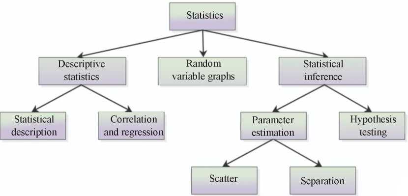
Fig. 1. Statistical control [2]
In case when the result of the process is influenced by many variables, to find such combinations of values of input variables that significantly affect the variability of output data through statistical methods is a challenge. And the most demanded is how to effectively manage a process or phenomenon to get the desired result at the output. Using data mining tools, it is much easier to find relationships between multidimensional input and output data. Data mining is very precisely defined by the very title of book [3] — “Discovering Knowledge in Data”. There is a definition of data mining, formulated in 2001, as the analysis of (often huge) sets of observational data to discover unexpected relationships and generalize the data in an original way so that they are understandable and useful to their owner [4–5].
For these needs, methods and algorithms are being developed, thanks to which the search for the above compounds is faster and more efficient. Data mining methods can be divided into:
— association detection (association rules);
— classification and prediction;
— grouping;
— sequence and time series analysis;
— detection of characteristics;
— text and semi-structured data mining;
— study of content posted on the Internet;
— study of graphs and social networks;
— intelligent analysis of multimedia and spatial data;
— outliers detection [6].
On this basis, methods commonly called artificial intelligence have been developed, through which the most frequently selected data mining tasks are performed. Despite the development of information technology and the increasing processing power of computers, it is still almost unfeasible to test all possible combinations of multidimensional input and output of a complex system [7]. The more complex the problem is and the mechanisms controlling it are unknown, the more justified the application of artificial intelligence methods is (Fig. 2).
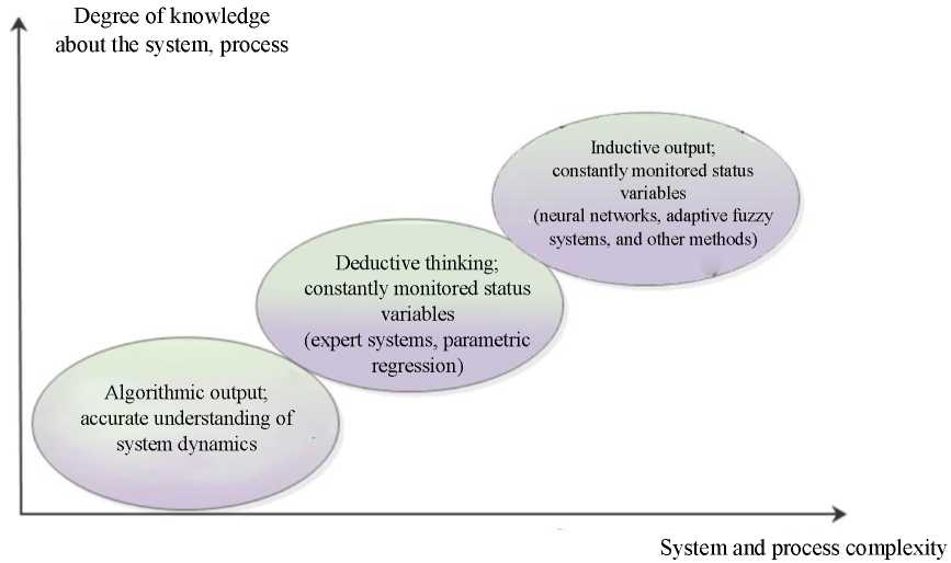
Fig. 2. Proposed conditions for application of artificial intelligence methods [7]
There are many methods and techniques of artificial intelligence (including artificial neural networks, the Knearest neighbor method, random forest, decision trees), and they are still being developed1. Popularity, which can be read as the usefulness of applications of one of the artificial intelligence tools — artificial neural networks — is very noticeable, e.g., based on [8]. Instead of a strict search for possible combinations, metaheuristics is used. If you want to apply the aforementioned tools, you should decide whether to use specialized software or create it yourself through publicly available modules (so-called “engines”) that implement artificial intelligence algorithms. Regardless of the decision taken, the basis will be the data that are analyzed.
Data preparation. The following stages of data preparation for analysis can be distinguished:
— data cleansing;
— data integration;
— data selection;
— data consolidation and transformation [6].
Such preparation should be performed regardless of the database size. Their proper preparation is even more important for small datasets than for large ones. An example is a comparison of two datasets: one with 10,000 records, and the other with 100 records, where 5 % of the records relate to a recurring phenomenon (repeatability has not yet been detected). When two records contain erroneous data, then in the first case, we can find repeatability in 4.8 % of cases instead of 5.0 %. In the second case, the repeatability is detected only in 3.0 %. The difference is significant.
Data cleansing and integration. When clearing data, records containing incomplete data are mostly deleted from the database. In large databases, deletion, e.g., of 2 records will not significantly affect the results obtained at subsequent stages. With a small number of datasets, the loss of even one record can significantly affect the analysis results obtained. For this reason, the missing values cannot be replaced, e.g., by the average for the entire population (one of the data augmentation methods) or its part (similar to the description in the record to be deleted), as is done for large databases. The reason is the same as described above — replacing one missing feature in the description of the phenomenon can significantly change the results if a small dataset is analyzed. However, records deleted in the process should not be permanently deleted. At subsequent stages, it may turn out that this feature will not be taken into account in the finally adopted model, and the initially deleted record will contain complete data — this will be useful for analysis.
The second important stage of data cleansing is a statistical analysis of each characteristic (columns in the database) separately and its correlation with the output data. It is recommended to present statistics of the major characteristics of the analyzed process (number of records, arithmetic mean, median, minimum and maximum values, standard deviation, quartiles of characteristic values) also for the function or functions describing the output data. “Boxand whisker” plots are very easy-to-follow (Fig. 3).
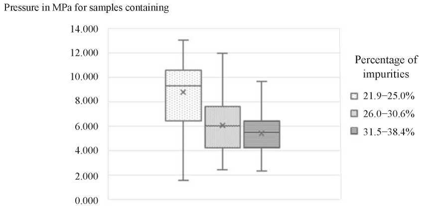
Fig. 3. Example of a “box-and-whisker” type diagram [9]
On such a chart, it is easy to read, e.g., that for 50 % of samples with 21.9–25.0 % clay content with dust, the strength was above 9 MPa, but the minimum strength for this type of samples was below 2 MPa. For such samples, the strength was below 6.5 MPa. The analysis of basic statistics can facilitate the decision to exclude from the analysis the records (i.e., samples or investigated phenomena) for which the measured values are incompatible with all other cases. Significant discrepancy may be the result of an erroneous measurement or the fact that the measurement was affected by another factor that was not taken into account at all (it was not taken into account, it was not measured in any of the cases). For these reasons, all records rejected from the database should be described, and the reasons for rejection should also be indicated [10].
Another case. You have discovered, e.g., that a decision to reject a record can be made only after all or part of the calculations have been performed. This is discussed in paper [11]: on the basis of sets of 95 accelerations of a standardized hammer (hitting the tested steel element), measured every 0.01 ms using artificial neural networks, an attempt was made to assign the tested steel element to one of nine classes (Fig. 4–5).
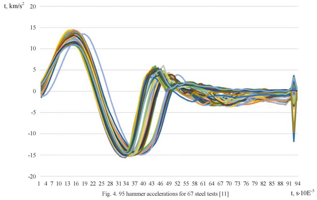
Analyzing the accelerations in Figure 4, we can say that one of the tests in the time range from 0.01 to 0.31 ms lags behind the others, but still behaves like other samples. Only the preliminary classification into four groups of steel grades showed that after 0.31 ms in test No. 29, results were obtained that show a sharply deviating nature of the results also after 0.31 ms (Fig. 5). In Test No. 29, a steel sample was examined, for which, in all other tests, acceleration changed the sign from negative to positive between 0.424 and 0.450 ms. For Test No. 29, the acceleration sign changed within 0.460–0.495 ms, i.e., in a time suitable for another group of steel grades. Only this conclusion allowed us to justify the deviation from the analyses of Test No. 29 well enough. Consequently, the initially obtained classification accuracy was increased to nine grades of steel according to the results of 67 tests, equal to 80 %, to 95 % (after excluding Test No. 29 and reusing artificial neural networks).

Fig. 5. Fragment of the diagram from Fig. 4 with a preliminary classification into four groups of steel classes and outlier Test No. 29 also after 0.31 ms [11]
Data integration is combining data on the same phenomenon from different sources into one database. An example of integration is presented in [12], which predicts a delay in the construction of sections of expressways and motorways in Poland. The independent variables on whose basis forecasts were made are data on the constructed facilities (prescribed by the Access to Information Act of the General Directorate for National Roads and Highways), data on enterprises implementing these facilities (collected in the Registration court), the Internet, the business intelligence agency, macroeconomic data (with a source in the publications of the Central Statistical Office). The dependent variable value (required for “training” an artificial neural network) is the number of days for which the completion of each of the analyzed road investments is postponed; it was searched for in publications in the press and on the Internet. The collected information was used for integrating the data on the implementation of 128 construction projects into the database. In Poland, 156 sections of expressways and motorways were built in 2009-2013, but it was almost impossible to get complete information on them. After analyzing this construction progress, those cases were rejected when unexpected violations occurred (e.g., in the form of protests by environmentalists, they were not taken into account in the analyses as an independent variable). This reduced the number of cases by 28, but provided the completeness and integrity of the database — the basis of the calculation.
Data selection. In large datasets, their size is a significant problem — a large number of records causes inefficient and long software performance. In databases with small record sizes, the search software for I/O relationships may not be sufficient to find those relationships. It happens that the phenomenon under study can be described by many parameters, but there are few cases (records) in the database with the described parameters of the phenomenon. Thus, the data selection means the need to choose only a few independent variables on whose basis the classification or prediction of the output value will be performed using artificial intelligence (also known as machine learning). When selecting independent variables, the following may be useful:
— study of the mutual correlation of linear independent variables, as well as the correlation with the values at the output;
— analysis of the main components;
— empirical search for the optimal set of independent variables.
Correlation research. The study of Pearson’s linear correlation between pairs of independent variables and between each of them and the dependent variable can be presented in the form of a table with numbers, as well as graphically, in the form of so-called “heat maps” (pairs of independent variables) [13]. The variables are most strongly correlated positively, and the intense blue color in Figure 6 shows the lowest value of the Pearson coefficient. A strong positive or negative correlation read from the heat map does not oblige to delete a variable that is highly correlated with another; this is just an assumption, because it strongly positively correlates with zn2 (the correlation coefficient between them is 0.88), and at the same time zn5 does not correlate with the output (denoted as wy, the correlation coefficient is 0.03).
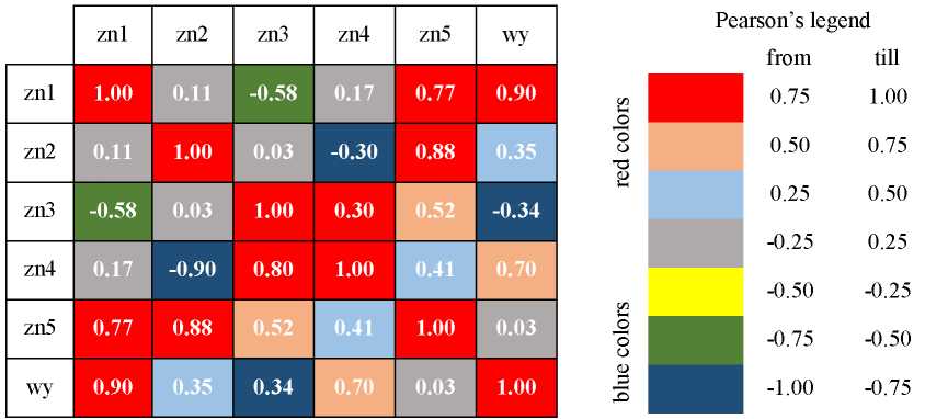
Fig. 6. Approximate “heat map” of independent variables from n1 to n5 and output data
Although linear correlation is computed, and the actual relationship between the independent variables (or the independent variable and the output-dependent variable) may not be linear, calculating these linear correlations often suggests which variables should not be included (if there is a need to reduce them). Such a check was made, among others, in [9][12]. In [12], the number of dependent variables was reduced, and in [9], a new variable was accepted for analysis as the sum of the values of two strongly positively correlated independent variables (this was also technically justified). A variable that has a strong negative correlation with another independent variable can also be removed from the database.
Principal component analysis. Principal component analysis (PCA) is performed for independent variables — the output value is not taken into account2. As a result, we obtain a rating showing which of the independent variables most affects the variability of sets of independent variables. Each of the independent variables can measure multidimensional space. Independent variables are interconnected, they form sets (records in the database describing the phenomenon). The PCA result is the answer to the question which of the independent variables is most responsible for the fact that the distances (in multidimensional space) between points (sets of independent variables described in the records — coordinates of points) are the largest. The variables that have the least impact on the data scattering are those that can be removed from the analysis in an attempt to reduce the number of independent variables. Examples of the effective application of the principal component analysis to improve the performance of machine learning tools can be easily found, e.g., in [14–16]. However, it should be borne in mind that PCA does not consider the value of the dependent variable. Thus, there is no certainty that it is the independent variable that also has the greatest impact on the predicted value (the dependent variable) that causes the greatest variability in the datasets.
Empirical research. Both the correlation study and the principal component analysis do not give absolute confidence whether the selection of independent variables was optimal. Optimal here means the most accurate prediction or the maximum possible proportion of accurate classifications for the database and the selected machine learning tool. Artificial intelligence tools are most often applied when their user suspects that there is a connection between input and output (between sets of independent variables and the effect of their joint occurrence — a dependent variable). When these dependences cannot be described strictly (by a function of many variables), when the studied processes and phenomena are complex (Fig. 2), then using machine learning tools may be the only way to find out about it. So, it is hard to expect that any auxiliary tool will accurately indicate which of the dependent variables should be used to “train” artificial intelligence. Hence, one of the methods of searching for the optimal set of input data (dependent variables) is the empirical verification of the results of an artificial intelligence tool on various sets of dependent variables. There are two main modes of action: forward and backward. “Forward” means selecting two dependent variables based on which the results of the prediction or classification are the best. It is sometimes very easy to choose the first one, but it is difficult to imagine a prediction of delays without specifying the planned duration [12][17]. To select the second variable, we check the operation of the tool on each created pair of dependent variables (they are sometimes called predictors) [18]. When the best pair of predictors is selected, one of the remaining predictors is added sequentially. This is done until adding some not-yet-used independent variable improves the results. In the backward procedure, the first step is to use all independent variables, and then remove sequentially only one, checking which predictor was removed, the accuracy of prediction and classification increased the most. The procedure continues until the removal of any of the predictors does not improve the results.
Data consolidation and transformation. The consolidation and transformation of data is so that it can be used by the selected data mining tool [6]. The most common form of data transformation is their standardization, i.e., such a transformation of the values of independent variables and dependent variable, in which they take values from the same range. Data standardization is the result of the need to provide each of the independent variables with a “level playing field” that will be included in the machine learning model. In [12], the formula is given:
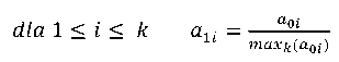 (1)
(1)
where 𝑘 — number of records in the database;
𝑎0𝑖 — i-th element of variable a before standardization;
𝑎1𝑖 — 𝑖𝑖-th element of variable a after standardization.
The second widely used type of data standardization is the so-called standardization “to zero mean and standard deviation of one” defined from the following formula:
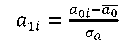 (2)
(2)
where — arithmetic mean of variable a before standardization;
𝑎0𝑖 — i-th element of variable a before standardization;
𝑎1𝑖 — i-th element of variable a after standardization;
𝜎0𝑎 — standard deviation of variable a before standardization [7].
Other types of standardization, also nonlinear, can be found, e.g., in [19]. However, it should be remembered that the type of data standardization can change the results obtained through machine learning [20]. Thus, the type of data standardization can be one of the parameters that the tool adjusts to get the best results.
Binarization can be the second data transformation process. It means converting the numeric values of a variable into only two values (e.g., 0 and 1) according to the following formula [22]:
 (3)
(3)
where 𝑎0𝑖 — i-th element of variable a before binarization,
𝑎1𝑖 — i-th element of variable a after binarization,
𝑝 — user-selected parameter.
Data binarization is especially useful when searching for rules applying market basket analysis (also known as association analysis)3. This type of analysis was created to investigate the contents of shopping carts to increase sales. Computer programs with the market basket analysis module work most effectively if the variables are binary (this product was present in the shopping carts or not). Many scientific problems can be formulated, whose very essence is binary, but in most cases, the description of the phenomenon includes numbers that are converted into binary form for the application of the market basket analysis [21–22]. Such transformation can also be performed for a variable that may belong to several disjoint subsets. Then, two dichotomous subsets (which are the sums of the original subsets) are created from the primary subsets. Then, if 𝑎0𝑖 belongs to one of them, then 𝑎1𝑖 is 0, if the other is 1.
Error measurements. So far, the author has used general terms such as “accuracy of predictions”, “correctness of classification”, which can be called the quality or effectiveness of artificial intelligence tools. However, if we analyze ways to improve the quality of their work, it is required to identify errors in the results of machine learning tools and the results of data mining.
Prediction errors. Machine learning tools mainly serve two purposes: to predict values (regression) and to carry out automatic classification. Using the same commonly accepted error measures facilitates understanding of work, but also makes it easier to assess the value of the prediction. It is assumed that the absolute value of the error is analyzed. Therefore, the absolute error (AE) [7][18] can be defined as
 (4)
(4)
where  — predicted value;
𝑏 — actual observed value.
Relative error expressed as absolute percentage error (APE), is defined as
 (5)
(5)
To be able to evaluate the quality of predictions made through an artificial intelligence tool (e.g., an artificial neural network), some data is not used in the “learning” process. After building the model, this dataset called a test sample is entered, and the machine makes predictions. So, the predicted values are a dozen, a few dozen or more. Then, to assess the quality of predictions, you can calculate the mean absolute percentage error (MAPE):
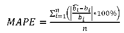 (6)
(6)
where n — size of the validation sample.
The most common error measure (check test) is the mean square error (MSE), defined as
 (7)
(7)
When solving regression problems, most machine learning tools, through the use of heuristic algorithms, search for input and output display that minimizes MSE. When specifying the quality of the predictions received, the most common are MSE or MAPE (or both). It should be noted that in case of MAPE, it does not matter whether this error is calculated for standardized or real values — MAPE is the same. This is not the case with MSE. This error most often has different values for standardized predictions and for predictions converted to true values (without standardization). Hence, it is required to specify for which values the MSE were calculated. Comparing the accuracy of predictions (different processes, phenomena with different instruments) based on MSE is feasible if MSE is calculated for standardized values. On the other hand, from the point of view of practical application, MAPE or the maximum value of AE is more important. The usefulness of the predictions obtained is also an important issue [24]. Predicting indirect construction costs with an average relative error of 6 % can be considered accurate and useful, but the same 6 % MAPE for stock market predictions makes them useless [24]. Thus, the size of the error obtained in the predictions should also be assessed from the point of view of usefulness for decision-makers using predictions.
Classification accuracy measures. When using machine learning tools for automatic classification, assignment of a case to the wrong class can be assessed in two ways. First, just as a mistake. However, the mere information that the tool correctly classifies 90 % of cases may not be enough. If there are multiple classes assigned to separate cases (described in the database) (e.g., 8), it may happen that for 5 classes, the classification is 100 % correct, and 10% of the errors are attributed to the other 3 classes. Hence, the quality of the classification results is assessed by the so-called error matrix (Table 1).
Table 1
Results of classification of tender procedures by validation sample [25]
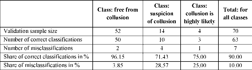
Significant differences in the classification accuracy of individual subsets may contribute to the further search for an even more accurate classification model. The error matrix may also contain information to which incorrect class this record from the validation sample was incorrectly assigned. This affects the forecasting inference. Analyzing the example from Table 1 with the following assumptions:
— 2 misclassified records from the “free from collusion” class assigned to the “suspicion of collusion” class by the automatic classifier;
— 4 misclassified cases from the “suspicion of collusion” class were assigned to the “highly likely collusion” class by the automatic classifier;
— 1 misclassified case from the “highly likely” class was assigned to the “suspicion of collusion” class by the automatic classifier, it can be stated that as long as the classifier does not assign this procedure to the “free from collusion” class, one can be sure that this production is not related to collusion. All cases assigned to this class were correctly classified by the automatic classifier (despite the classification accuracy of less than 100%). This effect was used, e.g., in [11]. Thus, it is worth analyzing which classes this case was automatically assigned to.
The classification error in medical applications is the division of errors into only two classes, where it is just as important not to administer medications to a healthy person as not to refuse treatment to a really sick person (mistaking him healthy) (Fig. 7).
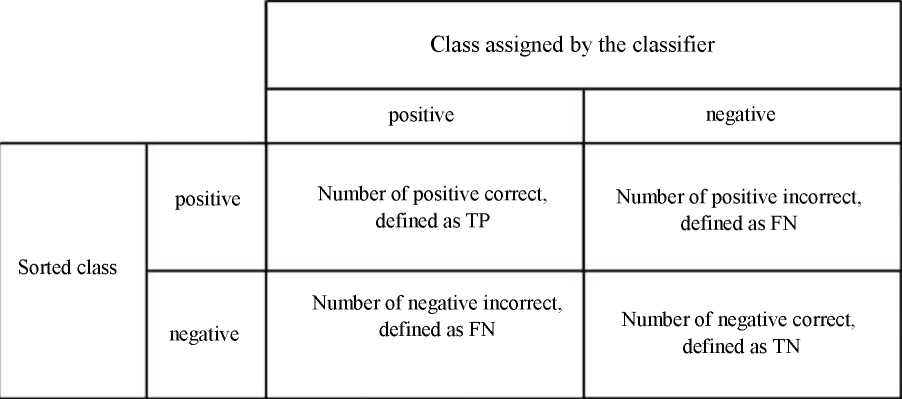
Fig. 7. Classification error matrix into two classes; gray background indicates correct classification4 [26]
For n classified cases, the following equality holds:
𝑛 = 𝑇P + 𝐹P + 𝑇N + 𝐹N (8)
To interpret the error matrix in the form shown in Figure 7, the concepts of accuracy, precision, sensitivity, specificity, are used; they are determined from the following equations5 [26]:
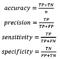
However, it should be remembered that the above indicators are applicable only if the tool classifies but two classes.
Determination of the significance of the discovered association rules. Through the market basket analysis (one of the mining tools), rules are discovered in the data that can be written as
𝑏 → ℎ (13)
where b — predecessor; h — successor of the rule.
This rule reads as follows: if there was a predecessor, then there was a successor. Both the predecessor and the successor may consist of several variables, but most often the rules are sought in which the predecessor is described by many variables, and the successor — by one (e.g., if the pressure dropped in the morning and the temperature at noon exceeded 30, then there was a thunderstorm in the afternoon). Such a rule (as in the example above) does not always work. Consequently, the quality measures of the discovered rules are not error measures, but three parameters (proportions) [6][9], through which it can be easily determined that the rule will be checked in case of violation of the predecessor [3][4][6]:
— support — marked as sup
— confidence — marked as conf;
— marked as lift
Support is defined as follows:
 (14)
(14)
where 𝑛(𝑏 → ℎ) — the number of cases in which the occurrence of a predecessor was accompanied by the occurrence of a successor; 𝑁 — the number of all cases in the database.
On the other hand, the validity of the rule is determined as follows:
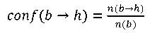 (15)
(15)
where 𝑛(𝑏) — the number of cases in which the occurrence of a predecessor was noted.
Equally important is a lift of the rule. If its value is less than 1, it means that the found rule does not explain the occurrence of a successor. Lift is defined as follows:
 (16)
(16)
where 𝑃(ℎ) — the likelihood of a successor (independent form the predecessor occurracne).
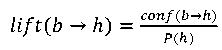
For a better understanding of the assessment of the quality of the association rules discovered, there is an example in which 10 observations were made in 12 processes for the occurrence of a predecessor and a successor (Fig. 8). For the rule “if a predecessor, then a successor “, support, confidence and lift (for each of the processes) were calculated (Table 2).
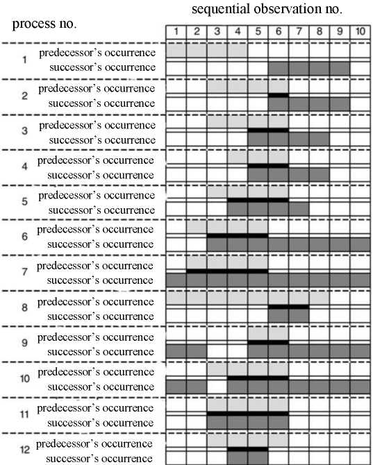
Fig. 8. Observing the occurrence of predecessor and successor in 12 processes
Source: own development
Comparing processes 5 and 6, it should be noted that a high degree of reliability of the rules is not always important. In process 6, a successor is almost always present, and the discovered rule does not explain the occurrence of the successor (lift<1). This does not apply to process 8. Lift indicates the importance of the rule, while its confidence is low. However, every observation of the successor is accompanied by an observation of the predecessor. In case of process 8, therefore, it is worth clarifying the predecessor (e.g., by adding another variable). In that event, probably, another parameter (not yet included in the predecessor) affects the presence of a successor (in process 8).
Table 2
Rule evaluation using sup, conf, and lift for the processes in Figure 8

Important aspects of applying selected tools of artificial intelligence and data mining to small databases
The number of records in the database and complexity of the tool. In statistics, it is most often assumed that a small sample size is less than 30 cases, but it can be found that the limit beyond which we cannot talk about a small sample is 100 [27−28]. Artificial intelligence tools need complete data sets (inputs and outputs) to be able to find the most accurate way to transform one into another. The more complex the problem, the more data sets (records in the database) are required. In deep learning, when a tool is taught not with sets of numbers, but with files (graphics, audio, text), thousands of data sets are needed. In [29], more than 4,000 standardized images were used to predict compressive strength. In other studies, there were few samples (e.g., in [11] there were only 66). There is an indication that for artificial neural networks, the number of connections between neurons should be 10 times less than the number of records in the database [30]. Small databases require more computational testing and finer tuning of the tools used. However, the rule that the more complex the problem and its model, the more data sets are required to train the tool, remains valid. The application of complex models (e.g., artificial neural networks with more than one hidden layer and many neurons in hidden layers) in small databases most often causes errors (prediction or classification), much greater than in models with less complexity of the tool itself. Hence the popularity of the methods of reducing the number of independent variables described in Section 3. When the number of datasets is too small, reducing the number of independent variables most often increases the accuracy of forecasts and classification.
Type of inference and quality of prediction and classification. Paper [30] suggests that artificial neural networks can more accurately determine whether, e.g., the predicted value will be greater than the value given by the network user. Referring to the requirement of the prediction usefulness [23], if the predictions obtained are not accurate enough (i.e., the prediction errors are too large), it is possible to decide whether an accurate value is required. When, e.g., predicting the strength of a material, it is possible, instead of a prediction, only to report that the strength will not be lower than the estimated strength specified by the user. It is the same with the classification problem. Automatic classification of steel into 9 grades based on a total of 66 entries in the database did not enable to obtain the classification accuracy above 80 % [11]. Then, one classification process was replaced by the eighth, as a result of which the steel test results were divided into two dichotomous subgroups, as shown in Fig. 9.
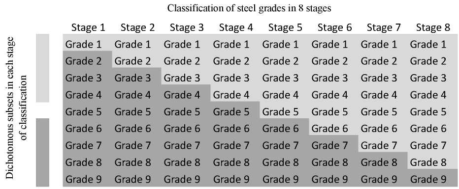
Fig. 9. Eight-stage classification process into 2 dichotomous subsets (at each stage of classification) [11]
Automatic classification of only two subsets was carried out using a simpler model (with complexity corresponding to the number of steel tests, i.e., 66). The process used eight times provided an increase in the classification accuracy from 80 to 95 %. In [12], out of the originally selected 12 predictors, only 6 remain. This made it possible to make a sufficiently small error prediction for the model to be useful. Computer programs enable to predict, e.g., 2 dependent variables at the same time; but for the above reasons, better results (smaller errors) are obtained when predicting 2 dependent variables separately, using 2 models, although the results are obtained on the same dataset.
Output modification. Let us consider the case when at the initial stage of calculations, sufficiently accurate predictions or classifications are not obtained. In addition to the actions related to data and complexity in the machine learning tool used above, we can consider the possibility of searching for another dependent variable, the one on whose basis it will be possible to calculate a strictly dependent variable that needs to be found. With a small number of records in the database, this can simplify the model, which, in turn, can increase the accuracy of predictions. This effect was used in [31], where an artificial neural network prediction is only part of the mixture design process. Another procedure that can reduce prediction errors is the prediction of a relative value (instead of an absolute value). When optimizing the operation in [12], the predicted delay expressed in days was replaced by a delay expressed as a proportion of the number of days of delay to the planned number of days of the construction. In this case, it did not reduce the errors in the predictions. Another possibility to change the type of output (i.e., the predicted dependent variable) is to replace one number with several values of membership functions calculated on the basis of fuzzy set theory [32]. In [17], instead of the number of days of the construction delay at the output of an artificial neural network, 3 values of the set membership function were used: low delay, medium delay and long delay. After clarifying the predicted values, it turned out that the prediction errors were less than when predicting the number of days of delay [12]. The same was done in [33] through predicting the values of the membership function at the first stage of calculations, and only at the second stage, based on these predictions, the cases were divided into 3 subsets. However, in this case, the direct application of an artificial neural network as a classifier caused an increase in the classification accuracy.
Hybrid tools. With a small number of cases in the database, the machine learning tool used cannot be very complex since there are too few cases to successfully train the model. Hybrid models can be a remedy for too big a prediction error or too low classification accuracy. Instead of one complex tool, two simpler ones are used. In the above example [17], the application of fuzzy set theory actually adds 2 elements to the model that can be properly “tuned”. The diagram of the model is shown in Figure 10.
Fig. 10. Three modules of the neuro-fuzzy model [17]
The first module is the conversion of exact numbers into the values of three membership functions. The second is to configure the network to predict these three values with the least error, and the third is to increase the accuracy of the obtained forecasts to exact numbers. Operations in each of these three modules can be performed differently, so, 3 tools can be used to model the dependent variable, and not just the artificial neural network itself. There is variety of examples when hybrid models, i.e., those in which more than one tool, are used together and make more accurate predictions than models with one tool [34–30]. Therefore, when analyzing research results, it is worth considering the possibility of using machine learning tools together with other mathematical tools.
Separation of the validation subset. To train artificial neural networks, from an existing database, three subsets are allocated, containing both independent and dependent variables: training, testing and validation. The training subset is used to train the tool. This process continues until the MSE stops decreasing in the test sample, then the network learning process stops. Further training of the network could lead to a better agreement of the tool with the training data, but the possibilities of generalization would be lost (the MSE errors for the test and test samples would be much higher) [30]. This effect, called artificial neural network overfitting, is schematically shown in Figure 12.
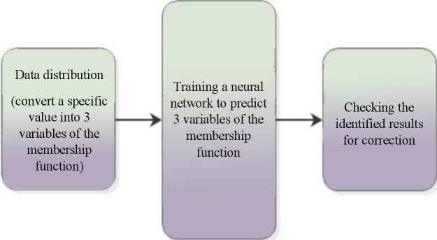
Fig. 12. Schematic of artificial neural network overfitting and correctly found trend [32–33]
A validation subset is used to assess the quality of predictions or classification. These sets of independent variables and the dependent variable do not see the network in the learning process. Therefore, predictions (or classifications) are made for a test subset, and the errors described in the previous sections can be calculated through comparing to the known dependent variables. It is critical to specify which subset the calculated error belongs to. One of the methods of assessing whether the tool is not overfitted is to compare errors (most often MSE) for the above three subsets, they should be at a similar level. Explicitly lower MSE for the training subset may indicate overfitting, and explicitly higher MSE may indicate a tool imperfection. Explicitly lower MSE for the test and validation sample implies the need to select other parameters of the artificial neural network or other dependent variables (or even another tool).
For large databases, a random division of data into three subsets is appropriate. There are suggestions in the literature that the proportions of the size of these subsets should be in the range of 60:20:20–70:15:15 (trainer: test: check) [36−37]. For small databases, random selection is only appropriate when different ranges of the dependent variable (or class for classification) are equally numerically represented. Most often, this condition is not met. Then it would be good to provide such a balanced representation in all 3 subsets. This controlled data separation was used in [11][25]. In [11], out of 66 tests of steel, one brand (5 tests) was the least numerous, and the brand with 12 tests was the most numerous. With a random selection of tests for subsets, it could happen that not a single test of any steel grade was included in the training subgroup, which would undoubtedly prevent its automatic recognition. In [25], out of 249 analyzed cases, only 9, according to the authors, should be classified as “highly likely collusion”. After partitioning the dataset into subsets, 4 of these procedures were assigned to the training one, 1 — to the test one, and 4 — to the validation one. With this procedure, 3 out of 4 procedures in the validation set can be correctly classified.
In the Polish and English-language literature, you can find examples of the authors using only the concepts of a training dataset, a test dataset. This probably happens for two reasons. Some computer programs completely (without user intervention) control whether the tool is overfitted. Then, only the validation set is extracted (either by specifying its quantity or percentage in the total data, or through selecting the records to be used for validation). In this case, a validation subset is often called a test subset. The second reason is that some machine learning tools (e.g., classification trees, C&RT trees6) are protected from overfitting in a different way than MSE control for a test sample. The quality of these tools can be checked using a test subset (just like a validation subset — without participating in the learning process of the tool). Usually, already when reading papers on machine learning, it comes out whether two or three subsets of data have been allocated, so the different nomenclature of the set used to assess the quality of work is not a problem.
Model quality check. Databases with a small number of records used to build a model based on machine learning make the model less stable (i.e., give significantly different errors) when replacing records between subsets (training, testing, and validation). To see if the constructed model works well with only a certain separation of data into subsets, it should be run on randomized subsets. Using suggestions on the proportion of data separation, they can be divided into 5–7 subsets, and as many model building processes should be performed as possible, so that training will take place at each iteration. This model quality check is called cross-validation (in English, cross-validation datasets are called “convolutions”). The MSE or MAPE errors are then averaged. If, however, errors in any dataset deviate significantly from the average value, you should seek the reason for this.
Regardless of the size of the database, error estimation should also be viewed through the prism of the usefulness of the results. Predictions with relatively large errors, phenomena that cannot be accurately described, can be very useful and considered important. On the other hand, predictions with the same MSE or MAPE of another phenomenon may not give any new information on the phenomenon being studied. Thus, in addition to numerical values of prediction accuracy or classification accuracy, it is important to refer to the phenomenon under study itself.
It is also critical to check whether another model has been built for the previously studied phenomenon. If so, then a link to these previous studies (regarding the level of errors obtained there) will also validate the quality of the new patented solution. If such models have not been created before, you can check the quality of the new solution through comparing the results to a much simpler model (e.g., based on Microsoft Excel with Solver add-in).
There is a question to which there is no clear answer yet: does a small number of datasets mean that the predictions, classifications and association rules obtained are irrelevant (precisely because of their small number)?
For example, a complex and strict rule with the following indexes: sup = 0,01, conf = 1, lift = 100 for a database with 10,000 records means that every time a particular predecessor occurs 100 times, the specified predecessor is always (sic!) the next one. The same rule for a database of 100 records means that there was only one unique case when the specified predecessor took place. In one case, you cannot talk about a rule, but you can talk about a case (randomness). However, even for a small database (e.g., with 100 records), a 100 % confidence rule supported by 3 cases may already indicate repeatability (provided that the increment for this rule is greater than one).
There are small databases, usually because they are small in themselves, because the preparation of larger ones is expensive and very time-consuming. Moreover, they can also be a consequence of the nature of the phenomenon (e.g., a limited number of objects constructed by the same company). In reality, these databases cannot be expanded (several times or several dozen times). Analyzing such databases under the conditions described in this chapter, may cause the emergence of new, as yet unrecognized dependences. Constructed, properly functioning models may not be directly applicable to other similar phenomena, but they can effectively indicate methods for finding common relationships in cases where the number of datasets is much larger. Unique association rules or unexpected automatic classifications may also indicate areas on which further research of the described phenomena should be focused.
Summary. The problems and issues discussed in the paper related to the search for relationships between multidimensional input and output data are presented in a small number of cases. This work, therefore, cannot be a comprehensive subject overview. The length of the paper and the author’s limited experience in applying machine learning and data mining methods do not allow describing most of the methods used. Calculation problems (mainly on small databases) contained in the works mentioned in the text and their solutions are systematized in such a way that the sequence of actions is observed: from database preparation to calculations, to discussion of the results. It is not possible to clearly state how many records in the database may indicate a “small” or “large” database. However, it can be said that at least several dozen records are required for the effective use of machine learning or data mining tools. Through applying appropriate procedures (input data development, model building), these tools can be used for successful modeling and studying phenomena described in only a few dozen cases. Based on the calculations carried out, it is possible to draw a reliable conclusion.
1. StatSoft. Internetowy Podręcznik Statystyki. URL: https://www.statsoft.pl/textbook/stathome.html (accessed: July 2020).
2. StatSoft. Internetowy Podręcznik Statystyki. URL: https://www.statsoft.pl/textbook/stathome.html (accessed: July 2020).
3. StatSoft. Internetowy Podręcznik Statystyki. URL: https://www.statsoft.pl/textbook/stathome.html (accessed: July 2020).
4. PQStat Statystyczne Oprogramowanie Obliczeniowe. Available from: https://pqstat.pl/?mod_f=diagnoza (assessed: July 2020). (In Polish)
5. PQStat Statystyczne Oprogramowanie Obliczeniowe. Id.
6. StatSoft. Internetowy Podręcznik Statystyki. URL: https://www.statsoft.pl/textbook/stathome.html (accessed: July 2020).
1. Lissowski, G. Podstawy statystyki dla socjologów. Opis statystyczny. Tom 1 / G. Lissowski, J. Haman, M. Jasiński. — Warszawa: Wydawnictwo Naukowe Scholar, 2011. — 223 p.
2. Stanisławek J. Podstawy statystyki: opis statystyczny, korelacja i regresja, rozkłady zmiennej losowej, wnioskowanie statystyczne / J. Stanisławek. — Warszawa: Oficyna Wydawnicza Politechniki Warszawskiej, 2010. — 212 p.
3. Larose, D. T. Discovering Knowledge in Data: An Introduction to Data Mining. 2nd ed. / D. T. Larose, C.D. Larose. — Hoboken, NJ, USA: Wiley-IEEE Press, 2016. — 309 p.
4. Larose, D. T. Metody I modele eksploracji danych / D.T. Larose. Warszaw: PWN, 2012. — 337 p.
5. Hand, D. Principles of Data Mining / D. Hand, H. Mannila, P. Smyth. — Cambridge, MA, USA: MIT Press, 2001. — 322 p.
6. Morzy, T. Eksploracja danych. Metody i algorytmy / T. Morzy. — Warszawa: PWN, 2013. — 533 p.
7. Bartkiewicz, W. Sztuczne sieci neuronowe. W: Zieliński JS. (red), Inteligentne systemy w zarządzaniu. Teoria i praktyka / W. Bartkiewicz. — Warszawa: PWN, 2000. — 348 p.
8. Rutkowski, L. Metody i techniki sztucznej inteligencji / L. Rutkowski. — Warszawa: PWN, 2012. — 449 p.
9. Doroshenko, A. Applying Artificial Neural Networks In Construction / A. Doroshenko // In: Proceedings of 2nd International Symposium on ARFEE 2019. — 2020. — Vol. 143. — P. 01029. https://doi.org/10.1051/e3sconf/202014301029
10. Feature Importance of Stabilised Rammed Earth Components Affecting the Compressive Strength Calculated with Explainable Artificial Intelligence Tools / H. Anysz, Ł. Brzozowski, W. Kretowicz, P. Narloch // Materials. — 2020. — Vol. 13. — P. 2317. https://doi.org/10.3390/ma13102317
11. Artificial Neural Networks in Classification of Steel Grades Based on Non-Destructive Tests / A. Beskopylny, A. Lyapin, H. Anysz, et al. // Materials. — 2020. — Vol. 13. — P. 2445. https://doi.org/10.3390/ma13112445
12. Anysz, H. Wykorzystanie sztucznych sieci neuronowych do oceny możliwości wystąpienia opóźnień w realizacji kontraktów budowlanych / H. Anysz. — Warszawa: Oficyna Wydawnicza Politechniki Warszawskiej, 2017. — 280 p.
13. Rabiej, M. Statystyka z programem Statistica / M. Rabiej. — Poland: Helion, Gliwice, 2012. — 344 p.
14. Mrówczyńska, M. Compression of results of geodetic displacement measurements using the PCA method and neural networks / M. Mrówczyńska, J. Sztubecki, A. Greinert // Measurement. — 2020. — Vol. 158. — P. 107693. https://doi.org/10.1016/j.measurement.2020.107693
15. Mohamad-Saleh, J. Improved Neural Network Performance Using Principal Component Analysis on Matlab / J. Mohamad-Saleh, B. C. Hoyle // International Journal of the Computer, the Internet and Management. — 2008. — Vol. 16. — P. 1–8.
16. Juszczyk, M. Application of PCA-based data compression in the ANN-supported conceptual cost estimation of residential buildings / M. Juszczyk // AIP Conference Proceedings. — 2016. — Vol. 1738. — P. 200007. https://doi.org/10.1063/1.4951979
17. Anysz, H. Neuro-fuzzy predictions of construction site completion dates / H. Anysz, N. Ibadov // Technical Transactions. Civil Engineering. — 2017. — Vol. 6. — P. 51–58. https://doi.org/10.4467/2353737XCT.17.086.6562
18. Rogalska, M. Wieloczynnikowe modele w prognozowaniu czasu procesów budowlanych / M. Rogalska. — Lublin: Politechniki Lubelskiej, 2016. — 154 p.
19. Kaftanowicz, M. Multiple-criteria analysis of plasterboard systems / M. Kaftanowicz, M. Krzemiński // Procedia Engineering. — 2015. — Vol. 111. — P. 351–355. https://doi.org/10.1016/j.proeng.2015.07.102
20. Anysz, H. The influence of input data standardization method on prediction accuracy of artificial neural networks / H. Anysz, A. Zbiciak, I. Ibadov // Procedia Engineering. — 2016. — Vol. 153. — P. 66–70. https://doi.org/10.1016/j.proeng.2016.08.081
21. Nicał, A. The quality management in precast concrete production and delivery processes supported by association analysis / A. Nicał, H. Anysz // International Journal of Environmental Science and Technology. — 2020. — Vol. 17. — P. 577–590. https://doi.org/10.1007/s13762-019-02597-9
22. Anysz, H. The association analysis for risk evaluation of significant delay occurrence in the completion date of construction project / H. Anysz, B. Buczkowski // International Journal of Environmental Science and Technology. — 2019. — Vol. 16. — P. 5396–5374. https://doi.org/10.1007/s13762-018-1892-7
23. Zeliaś, A. Prognozowanie ekonomiczne. Teoria, przykłady, zadania / A. Zeliaś, B. Pawełek, S. Wanat. — Warszawa: PWN, 2013. — 380 p.
24. Juszczyk, M. Modelling Construction Site Cost Index Based on Neural Network Ensembles/ M. Juszczyk, A. Leśniak // Symmetry. — 2019. — Vol. 11. — P. 411. https://doi.org/10.3390/sym11030411
25. Anysz, H. Comparison of ANN Classifier to the Neuro-Fuzzy System for Collusion Detection in the Tender Procedures of Road Construction Sector / H. Anysz, A. Foremny, J. Kulejewski // IOP Conference Series: Materials Science and Engineering. — 2019. — Vol. 471. — P. 112064. https://doi.org/10.1088/1757- 899X/471/11/112064
26. Piegorsch, W. W. Confusion Matrix. In: Wiley StatsRef: Statistics Reference Online. — 2020. — P. 1–4. https://doi.org/10.1002/9781118445112.stat08244
27. Kot, S. M. Statystyka / S. M. Kot, J. Jakubowski, A. Sokołowski. — Warszawa: DIFIN, 2011. — 528 p.
28. Aczel, A. D. Statystyka w zarządzaniu / A. D. Aczel, J. Saunderpandian. — Warszawa: PWN, 2000. — 977 p.
29. Narloch, P. Predicting Compressive Strength of Cement-Stabilized Rammed Earth Based on SEM Images Using Computer Vision and Deep Learning / P. Narloch, A. Hassanat, A. S. Trawneh, et al. // Applied Sciences, 2019. — Vol. 9. — P. 5131. https://doi.org/10.3390/app9235131
30. Tadeusiewicz, R. Sieci neuronowe / R. Tadeusiewicz. — Kraków: Akademicka Oficyna Wydawnicza, 1993. — 130 p.
31. Anysz, H. Designing the Composition of Cement Stabilized Rammed Earth Using Artificial Neural Networks / H. Anysz, P. Narloch // Materials. — 2019. — Vol. 12. — P. 1396. https://doi.org/10.3390/ma12091396
32. Zadeh, L. A. Fuzzy Sets / L. A. Zadeh // Information and Control. — 1965. — Vol. 8. — P. 338–353. https://doi.org/10.1016/S0019-9958(65)90241-X
33. Yagang Zhang. A hybrid prediction model for forecasting wind energy resources / Yagang Zhang, Guifang Pan // Environmental Science and Pollution Research. — 2020. — Vol. 27. — P. 19428–19446. https://doi.org/10.1007/s11356-020-08452-6
34. Eugene, E.A. Learning and Optimization with Bayesian Hybrid Models. 2020 American Control Conference (ACC) / E. A. Eugene, Xian Gao, A. W. Dowling. — IEEE. — 2020. https://doi.org/10.23919/ACC45564.2020.9148007
35. Neural Network Design / M. T. Hagan, H. B. Demuth, M. H. Beale, O. De Jesús. — Martin Hagan: Lexington, KY, USA, 2014. — 1012 p.
36. Osowski, S. Sieci neuronowe do przetwarzania informacji / S. Osowski. —Warszawa: Oficyna Wydawnicza PW, 2006. — 419 p.
Anysz H. Machine Learning and data mining tools applied for databases of low number of records. Advanced Engineering Research (Rostov-on-Don). 2021;21(4):346-363. https://doi.org/10.23947/2687-1653-2021-21-4-346-363


Advanced Engineering Research (Rostov-on-Don)
ISSN 2687-1653 (Online)
Contact with: Publisher / Editorial Office of the Journal
Publisher: Don State Technical University - DSTU, Rostov-on-Don, Russia - https://donstu.ru/en/
Editor-in-Chief: Alexey N. Beskopylny, Dr.Sci. (Eng.), Professor, Vice-Rector, Don State Technical University (Rostov-on-Don, Russia)
Don State Technical University
1, Gagarin Sq., Rostov-on-Don, 344003, Russia
tel.: +7 (863) 2738-372, e-mail: vestnik@donstu.ru
16+
Processing of personal data