Contents
Scroll to:
https://doi.org/10.23947/2687-1653-2021-21-4-300-307
Scroll to:
Introduction. The concept of estimating the dynamic parameters of the “base — weakened layer — block” system is proposed, taking into account the physical nonlinearity of the material and the kinematic method of excitation of vibrations. In accordance with this approach, the physical nonlinearity of the base and block material is considered using the Drucker- Prager model. The weakened layer is modeled by 3D spring finite elements. The verification procedure of the proposed methodology is carried out on the example of the dynamic calculation of the “base — weakened layer — slope” system.
Materials and Methods. The computational experiments were performed using the ANSYS Mechanical software package in combination with a nonlinear solver based on the Newton-Raphson procedure. SOLID45 volumetric finite elements were used to discretize the computational domains. Combined elastic-viscous elements COMBIN14 were used to simulate the displacement of the block relative to the fixed base.
Results. An engineering technique for the dynamic analysis of the stress-strain state of the “base — weakened layer — block” spatial system with kinematic method of excitation of vibrations is developed. The accuracy and convergence of the proposed method is investigated using specific numerical examples.
Discussion and Conclusion. Based on the mathematic simulation performed, it is shown that the developed technique provides assessing the risks of the occurrence of real landslide processes caused by external non-stationary impacts.
Gaidzhurov P.P., Saveleva N.A., Trufanova E.V. Numerical simulation of the behavior of kinematically unstable slopes under dynamic influences. Advanced Engineering Research (Rostov-on-Don). 2021;21(4):300-307. https://doi.org/10.23947/2687-1653-2021-21-4-300-307
Introduction. In the 70s of the last century, the finite element method (FEM) began to be extensively used in the analysis of the static stability of slopes and flanks [1–3]. According to the practice of geotechnical calculations, FEM, in contrast to simplified methods, provided taking into account such important factors as the real geometry and layered structure of the objects under study, as well as the presence of anti-landslide structures and the physical nonlinearity of the material with a previously unknown area of plasticity [4]. Currently, many researchers start using FEM to analyze the dynamic stability of actual slopes, as well as forecasting the risks of rock falls in the underground workings and from slopes located along highways and railways. Also, one of the topical areas of mountain dynamics is finite element modeling of earthquake consequences, taking into account the kinematic instability of conglomerations [5]. Today, there are the following methods of dynamic calculations in the field of geotechnics:
1. SRM (strength reduction method) is a method of reducing strength [6, 7]. It is designed to calculate the safety margin of a mountain range in a physically nonlinear formulation. In SRM, the actual strength parameters of the soil are iteratively reduced through dividing by some factor greater than 1:
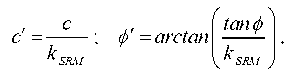
where c, ф — actual values of the adhesion and the angle of internal friction of the soil, respectively;  — the adhesion and the angle of internal friction of the soil, respectively, after their reduction relative to the actual values; kSRM — the shear strength reduction factor. Value kSRM, corresponding to the limiting state of the system, determines the lower limit of the strength parameters of the material.
2. LEM (limit equilibrium method) is a method of limiting kinetics based on D'Alembert's principle [8][9]. It is focused on the analysis of dynamic stability of articulated rock massifs.
3. TLEM (thin layer element method of FEM) is a thin-layer finite element method [10] in which elastic-plastic elements of a thin layer are used to model the behavior of kinematically unstable structures.
Analysis of the results obtained using the SRM, LEM and TLEM methods showed that there is currently no unified vision of mathematical modeling of the behavior of structurally unstable geotechnical systems under nonstationary external influence. This determines the topicality of developing a methodology for dynamic analysis of systems of the “base — weakened layer — block” type in a finite element formulation through a new approach to simulating sliding planes.
Materials and Methods. The equation of motion of a mechanical system in a finite element formulation can be given as follows [11]:
 (1)
(1)
where [M], [C], [K] — matrices of masses, damping and stiffness of the ensemble of finite elements, respectively;
 — vectors-columns, respectively, of nodal accelerations, velocities, displacements;
 — vectors-columns of specified static and dynamic loads, respectively, at a time t. In the future, we assume that the matrices [M] and [K] are consistent.
For the numerical integration of equation (1), we use Newmark method [12]. Here, we assign the integration step along the time axis  t so that the contributions of physically significant proper pairs are considered with sufficient accuracy. In the future, we will consider the kinematic methods of excitation of vibrations, set using either model seismogram
  , or model accelerogram
  . With this method of setting the dynamic effect, the second term of the right side of equation (1) will be zero:
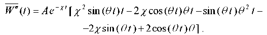
Consider the method of excitation of mechanical vibrations from a model seismogram. Function can be written as [13]:
 , (2)
, (2)
where A — initial amplitude;  — attenuation coefficient;
  — angular frequency of external influence. Figure 1 shows a graph of function
  for the values: A = 0,01553 m; = 0,7143; = 5 s–1.
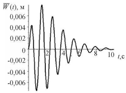
Fig. 1. Graph of the model seismogram
Research Results. As the first model example, consider the problem on forced vibrations of the slope located on the base (Fig. 2). The boundary conditions of the problem are shown in Figure 3, where letter S denotes the point under study.
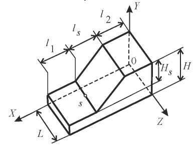
Fig. 2. Slope geometry
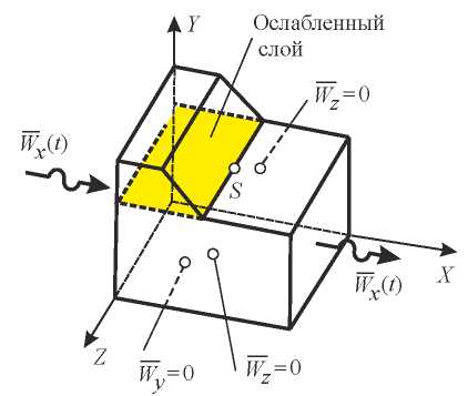
Fig. 3. Design scheme of the slope
Relationships between the geometric parameters of the slope and the base (Fig. 2) are presented in Table 1.
Table 1
Slope – Base Geometrics Relationship

Mechanical characteristics of the slope and base material are ae follows: deformation modulus Е = 21 MPa; Poisson's ratio v = 0.3; specific gravity y = 1702 кг/м3; adhesion с = 45 кПа; internal friction angle ф = 15°.
To model the slope and the base, we use SOLID45 volumetric finite elements of the ANSYS Mechanical software package. The finite element model for the variant with the parameters: ls = 2Hs, Hs = 10 m, assigned to the global Cartesian coordinate system, is shown in Figure 4.
The finite element grid is constructed so that on the contact surface, adjacent nodes of the base and slope have the same coordinates, but different numbers. This is done in order to arrange a weakened layer in this place. The kinematic effect in the form of a model seismogram (2) is set at each integration step ti in the form of nodal displacements  on the end surfaces of the model with parameters: X = 0 and X=l1 + ls + l2.
Modeling of the weakened layer (Fig. 4) is performed using elastic-viscous combined finite elements COMBIN14 [14]. The two-node element COMBIN14, consisting of a spring with stiffness k and a liquid friction damper with a damping coefficient сv, is shown in Figure 5. In the case under consideration, this element works only for tensioncompression.
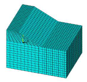
Fig. 4. Finite element model of the “base – slope” system
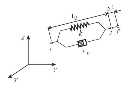
Fig. 5. Combined finite element COMBIN14
In each node of the contact surface (Fig. 4), along the global X, Y, Z axes, we introduce elements of COMBIN14. Parameters of combined elements are:
k = 30 кН/м; ky = kz = 9,44∙10 7 кN/m; сv = 0,5.
In this example, we further introduce the assumption of the natural undeformed state of the “base — weakened layer — slope” system. For calculations, we use the nonlinear solver of the ANSYS Mechanical complex.
The finite element modeling results in the form of visualization of the deformed state of the “base — slope” system with the account of the maximum horizontal displacement and the distribution of amplitude horizontal displacements Wx(t) are shown in Figures 6 and 7. The integration step of equation (1)  t = 0,01 s. As can be seen, the introduction of 3D elastic-viscous elements makes it possible to simulate the effect of kinematic instability of the “base — weakened layer — slope” mechanical system with the kinematic method of excitation of vibrations.
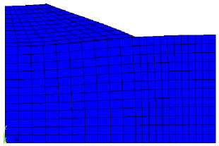
Fig. 6. Visualization of slope displacement regarding the base
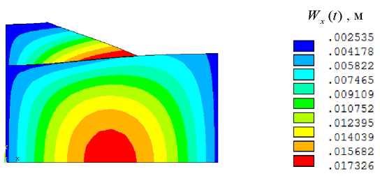
Fig. 7. Displacement distribution Wx(t)
The amplitude value of the displacement at point S was WxS max = 1,7 cm. For the slope option ls = Hs (fig. 2) WxS max = 1,1 cm. The graphs of base and slope vibrations at the studied point S (Fig. 3) in the direction of X-axis are shown in Figure 8.
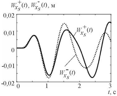
Fig. 8. Graphs of vibrations at point S of base  and slope
  under kinematic excitation using a model seismogram
Based on the above graphs, it can be seen that starting from the moment of time t > 1.5 s, there is a mismatch of base and slope vibrations.
Let us consider the behavior of the “base — weakened layer — slope” system (Fig. 3) when vibrations are excited using a model accelerogram  . To this end, we differentiate expression (2) twice. As a result, we get:
 (3)
(3)
Figure 9 shows the graph of function (3) for parameters: A = 0,01553 m; X = 0,7143;  = 5 s–1.
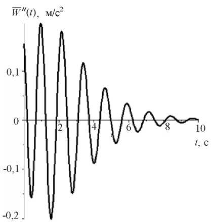
Fig. 9. Graph of the model accelerogram
The kinematic effect in the form of model accelerogram (3) , by analogy with seismogram (2), is set at each integration step ti in the form of nodal accelerations on the end surfaces of the model with parameters: X = 0 and X=l1 + ls + l2. Figure 10 shows the graphs of vibrations at the studied point S (Fig. 3) under kinematic action in the form of a model accelerogram. Comparing the vibration graphs shown in Figures 8 and 10, we establish that they almost coincide. This indicates the correctness of the developed finite element model, which allows describing the behavior of the “base — weakened layer — slope” system with various methods of unsteady kinematic action.
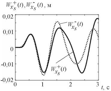
Fig. 10. Vibration graphs at point S of base  and slope
  under kinematic excitation of vibrations using a model accelerogram
As a second model example, let us consider the problem on forced slope vibrations with a kinematically unstable wedge-shaped inclusion (Fig. 11). Due to the symmetry of the configuration, only 1/2 part of the slope and inclusions are taken into account in the computational scheme. The boundary conditions for the accepted design scheme are shown in Figure 12. Here, letter S denotes the point under study, which belongs simultaneously to the slope base and the wedgeshaped inclusion.
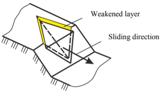
Fig. 11. Slope diagram with wedge-shaped inclusion
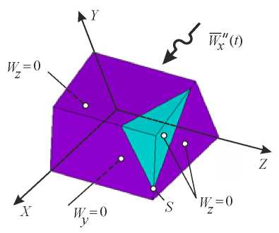
Fig. 12. Computational scheme for the “slope — wedgeshaped inclusion” problem
The finite element model of slope and wedge-shaped inclusion is shown in Figure 13. As in the previous example, in this case, we use SOLID45 and COMBIN14 elements with the same material characteristics.
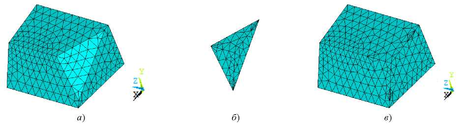
Fig. 13. Finite element model: a) slope; b) wedge-shaped inclusion; c) slope with wedge-shaped inclusion
The function describing the model accelerogram has the form:
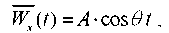
where A — acceleration amplitude;  — frequency of external influence. Figure 14 shows graph
  at A = 2,5 m/s2, = 2 Hz. The values of acceleration
  at the i-th step of integrating the equation of motion (1) are applied to the nodes of the model surface with coordinate X = 0 (Fig. 12).
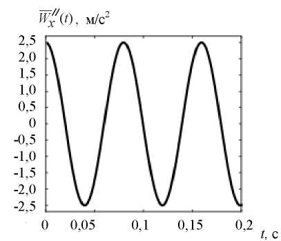
Fig. 14. Graph of the model accelerogram 
The simulation result in the form of a distribution of the amplitude values of displacements Wx (t) is shown in Figure 15. Integration step  t = 0,01 s. Vibration graphs of the slope base and wedge-shaped inclusion at the studied point S (Fig. 12) in the direction of X-axis are shown in Figure 16.
As can be seen from Figure 15, with a given kinematic effect, the continuity of the slope array breaks along the weakened layer, and the wedge-shaped inclusion shifts relative to the slope base along X-axis.
Fig. 15. Distributions Wx (t) in 1/2 part of the slope with wedge-shaped inclusion
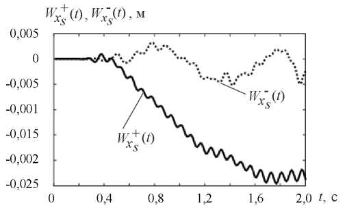
Fig. 16. Vibration graphs at point S of the slope base  and wedge-shaped inclusion
  under kinematic excitation of vibrations using a model accelerogram
“Drift” in Figure 16 is due to the fact that this finite element model has no connections that prevent displacements along X-axis. As shown in [11], it is possible to solve the “drift” problem by subtracting the displacement of the slope base, which represents the displacement “as a rigid whole”, from the displacement values and . It should be noted that the obtained amplitude values of the displacements provide evaluating the dynamic parameters of the “slope — weakened layer — wedge-shaped inclusion” system.
Conclusion. A finite element model has been developed and validated to study the dynamic behavior of kinematically unstable slopes in a three-dimensional formulation, taking into account the physical nonlinearity of the material.
1. Фадеев, А. Б. Метод конечных элементов в геомеханике / А. Б. Фадеев. — Москва : Недра, 1987. — 221 с.
2. Eberhardt, E. Rock Slope Stability Analysis – Utilization of Advanced Numerical Techniques / Erik Eberhardt. — Vancouver, Canada: Geological Engineering/Earth Ocean Sciences, UBS, 2003. — 41 p.
3. Hoek, H. Rock Slope Engineering. 3rd ed. / H. Hoek, J. W. Bray. — London: The Institution of Mining and Metallurgy, 1981. — 358 p.
4. Griffiths, D. V. Slope stability analysis by finite elements / D. V. Griffiths, P. A. Lane // Geotechnique. — 1999. — Vol. 49. — P. 387–403. https://doi.org/10.1680/geot.1999.49.3.387
5. Stability Modeling with SLOPE/W. An Engineering Methodology. — Alberta, Canada, 2015. — 244 p.
6. Tamotsu Matsui. Finite element slope stability analysis by shear strength reduction technique / Tamotsu Matsui, Ka-Ching San // Soils and Foundations. — 1992. — Vol. 32. — P. 59–70. https://doi.org/10.3208/sandf1972.32.59
7. Griffiths, D. V. Three-dimensional slope stability analysis by elasto-plastic finite elements / D. V. Griffiths, R. M. Marquez // Geotechnique. — 2007. — Vol. 57. — P. 537–546. https://doi.org/10.1680/geot.2007.57.6.537
8. Weida Ni. Dynamic Stability Analysis of Wedge in Rock Slope Based on Kinetic Vector Method / Weida Ni, Huiming Tang, Xiao Liu, et al. // Journal of Earth Science. — 2014. — Vol. 25. — P. 749–756.
9. Md. Moniruzzaman Moni. Stability analysis of slopes with surcharge by LEM and FEM / Md. Moniruzzaman Moni, Md. Mahmud Sazzad // International Journal of Advanced Structures and Geotechnical Engineering. — 2015. — Vol. 4. — P. 216–225.
10. Tongchun Li. Strength Reduction Method for Stability Analysis of Local Discontinuous Rock Mass with Iterative Method of Partitioned Finite Element and Interface Boundary Element / Tongchun Li, Jinwen He, Zhao Lanhao, et al. // Mathematical Problems in Engineering. — 2015. — Vol. 2015. — P. 1–11. https://doi.org/10.1155/2015/872834
11. Гайджуров, П. П. Моделирование динамического отклика системы «основание — фундамент — верхнее строение» при различных способах кинематического возбуждения колебаний / П. П. Гайджуров, А. В. Сазонова, Н. А. Савельева // Известия вузов. Северо-Кавказский регион. Технические науки. — 2019. — № 1 (201). — С. 23–30. https://doi.org/10.17213/0321-2653-2019-1-23-30
12. Бате, К. Численные методы анализа и метод конечных элементов / К. Бате, Е. М. Вилсон. — Москва : Стройиздат, 1982. — 448 с.
13. Сейсмостойкое строительство зданий / И. Л. Корчинский, Л. А. Бородин, А. Б. Гроссман [и. др.]. — Москва : Высшая школа, 1971. — 320 с.
14. Гайждуров, П. П. Конечно-элементное моделирование совместной работы оползня скольжения и защитного сооружения / П. П. Гайждуров, Н. А. Савельева, В. А. Дьяченков // Advanced Engineering Research. — 2021. — Т. 21, № 2. — С. 133–142. https://doi.org/10.23947/2687-1653-2021-21-2-133-142
Rostov-on-Don
Rostov-on-Don
Rostov-on-Don
Gaidzhurov P.P., Saveleva N.A., Trufanova E.V. Numerical simulation of the behavior of kinematically unstable slopes under dynamic influences. Advanced Engineering Research (Rostov-on-Don). 2021;21(4):300-307. https://doi.org/10.23947/2687-1653-2021-21-4-300-307


Advanced Engineering Research (Rostov-on-Don)
ISSN 2687-1653 (Online)
Contact with: Publisher / Editorial Office of the Journal
Publisher: Don State Technical University - DSTU, Rostov-on-Don, Russia - https://donstu.ru/en/
Editor-in-Chief: Alexey N. Beskopylny, Dr.Sci. (Eng.), Professor, Vice-Rector, Don State Technical University (Rostov-on-Don, Russia)
Don State Technical University
1, Gagarin Sq., Rostov-on-Don, 344003, Russia
tel.: +7 (863) 2738-372, e-mail: vestnik@donstu.ru
16+
Processing of personal data