Contents
Scroll to:
https://doi.org/10.23947/2687-1653-2023-23-3-329-339
Scroll to:
Introduction. Environmental problems arising in shallow waters and caused by both natural and man-made factors annually do significant damage to aquatic systems and coastal territories. It is possible to identify these problems in a timely manner, as well as ways to eliminate them, using modern computing systems. But earlier studies have shown that the resources of computing systems using only a central processor are not enough to solve large scientific problems, in particular, to predict major environmental accidents, assess the damage caused by them, and determine the possibilities of their elimination. For these purposes, it is proposed to use models of the computing system and decomposition of the computational domain to develop an algorithm for parallel-pipeline calculations. The research objective was to create a model of a parallel-conveyor computational process for solving a system of grid equations by a modified alternating-triangular iterative method using the decomposition of a three-dimensional uniform computational grid that takes into account technical characteristics of the equipment used for calculations.
Materials and Methods. Mathematical models of the computer system and computational grid were developed. The decomposition model of the computational domain was made taking into account the characteristics of a heterogeneous system. A parallel-pipeline method for solving a system of grid equations by a modified alternating-triangular iterative method was proposed.
Results. A program was written in the CUDA C language that implemented a parallel-pipeline method for solving a system of grid equations by a modified alternating-triangular iterative method. The experiments performed showed that with an increase in the number of threads, the computation time decreased, and when decomposing the computational grid, it was rational to split into fragments along coordinate z by a value not exceeding 10. The results of the experiments proved the efficiency of the developed parallel-pipeline method.
Discussion and Conclusion. As a result of the research, a model of a parallel-pipeline computing process was developed using the example of one of the most time-consuming stages of solving a system of grid equations by a modified alternating-triangular iterative method. Its construction was based on decomposition models of a three-dimensional uniform computational grid, which took into account the technical characteristics of the equipment used in the calculations. This program can provide you for the acceleration of the calculation process and even loading of program flows in time. The conducted numerical experiments validated the mathematical model of decomposition of the computational domain.
Litvinov V.N., Rudenko N.B., Gracheva N.N. Model of a Parallel-Pipeline Computational Process for Solving a System of Grid Equations. Advanced Engineering Research (Rostov-on-Don). 2023;23(3):329-339. https://doi.org/10.23947/2687-1653-2023-23-3-329-339
Introduction. Recently, a number of serious environmental problems have been observed in the Rostov region. These include, in particular, the eutrophication of waters of the Sea of Azov and the Tsimlyansk reservoir, which causes the growth of harmful and toxic species of phytoplankton populations [1]. Engineering works in the waters of rivers and seas cause pollution of adjacent territories, changes in the population structure of biota, and deterioration of reproduction conditions of valuable and commercial fish. Climate change in the south of Russia has led to an increase in the number of cases of flooding of some territories in the area of the Taganrog Bay and the floodplain of the Don River caused by up and down surges. In the last decade, during the summer period, almost complete drainage of the Don riverbed was observed several times, which led to a complete stop of navigation. To predict the occurrence and development of such cases, to plan ways to address their consequences, to assess the damage caused by them, modern software systems built using high-precision mathematical models, numerical methods, algorithms and data structures are needed [2].
Mathematical models used in predicting natural and man-made disasters are based on systems of partial differential equations, such as Poisson, Navier-Stokes, diffusion-convection-reaction, and thermal conductivity equations. The numerical solution to such systems causes the need for operational storage of large amounts of data (in arrays of various structures) and the solution to systems of grid equations of high dimension exceeding 109. The amount of RAM required to store arrays of data when numerically solving only one Poisson equation for a three-dimensional domain with a dimension of 103×103×103 by an alternately triangular iterative method is more than 64 GB. In the case of numerical solution to combined tasks, hundreds of gigabytes of RAM are required, which can be accessed only when using supercomputer systems.
An earlier study has shown that the resources of a computing system using only the CPU are not enough to solve such scientific problems [3]. Increasing the GPU power and video memory made it possible to use video adapter resources for calculations [4]. The GPU utilization depends on the application of parallel algorithms to solve computationally intensive problems of aquatic ecology [5–7]. To partially solve the problems of lack of memory and computing power on workstations, you can install additional video adapters in PCI-E X16 slots directly and in PCI-E X1 slots using PCI-E X1–PCI-E X16 adapters. Thus, the number of video adapters installed on one workstation can be increased to 12 [8–11].
Heterogeneous computer systems that provide sharing CPU and GPU resources are becoming increasingly popular in the scientific community. Application of such systems makes it possible to reduce the computation time of scientific problems [12–14]. However, the utilization of a heterogeneous computing environment involves the modernization of mathematical models, algorithms and programs that implement them numerically. A heterogeneous system provides organizing the calculation process in parallel mode. At the same time, fundamental differences in the construction of software systems using CPU and GPU together should be taken into account.
Materials and Methods. We describe the proposed mathematical models of the computational system, the computational grid, as well as the method of decomposition of the computational domain.
Let  be a set of technical characteristics of a computing system, then
 (1)
(1)
where
 — a subset of the characteristics of the central processing units (CPU) of a computing system;
 — a subset of the characteristics of video adapters (GPU) of a computing system;
 — a subset of RAM characteristics.
 (2)
(2)
where
 — total number of CPU cores;
 — number of streams simultaneously processed by one CPU core;
 — clock rate, MHz;
 — CPU bus frequency, MHz.
 , (3)
, (3)
where
 — multiple video adapter indices;
 — number of computer system video adapters;
 — video adapter index. Each video adapter is represented as a tuple
 , (4)
, (4)
where
 — amount of video memory of the video adapter with index
  , GB;
, GB;
 — number of streaming multiprocessors.
 , (5)
, (5)
where
 — total amount of RAM, GB;
 — clock rate of RAM, MHz.
Let  — a set of software streams involved in the computing process, then
 (6)
(6)
where
 — a subset of program streams implementing the calculation process on the CPU;
 — a subset of CUDA streaming blocks implementing the calculation process on GPU streaming multiprocessors;
 — number of CPU program streams involved;
 — a subset of CUDA streaming blocks that implement the calculation process on GPU streaming multiprocessors with index
  ;
;
 — multiple GPU indices;
 — number of GPU in the computing system;
 — number of CUDA stream blocks involved that implement the calculation process on GPU stream multiprocessors with index
  .
.
Let  be a set of identifiers of program streams. Then, in order to identify program flows in the computing system, we assign tuple
  of two elements to each element of the set of program flows S:
 , (7)
, (7)
where
 — index of a computing device in a computing system;
 — index of the CPU program stream or GPU streaming unit.
 , (8)
, (8)
 . (9)
. (9)
Let us take the computational domain with the following parameters:
 — characteristic size on axis
  ;
;
 — on axis
  ;
;
 — on axis
  .
.
We compare a uniform computational grid of the following type to the specified area:
 (10)
(10)
where
 ,
,  ,
,  — steps of the computational grid in the corresponding spatial directions;
 ,
,  ,
,  — number of nodes of the computational grid in the corresponding spatial directions.
Then, we represent the set of nodes of the computational grid in the form
 (11)
(11)
where  — computational grid node.
The number of nodes of the computational grid  is calculated from formula
 . (12)
By the subsection of the computational grid  (hereinafter — subsection), we mean a subset of the nodes of the computational grid
  .
.
 , (13)
where
 — multiple indices of subsections
  of computational grid
  ;
;
 — number of subsections
  ;
;
 ;
;
 — set of natural numbers;
 — index of subsection
  .
.
Since  , then
 , (14)
where
 — node of subsection
  ;
;
sign  indicates belonging to the subsection;
 — node index of subsection
  by coordinate
  ;
;
 — number of nodes in subsection
  by coordinate
  .
.
 (15)
(15)
where  — number of nodes by coordinate
  of
of  -th subsection.
Under the block of computational grid  (hereinafter — block), we mean a subset of the computational grid nodes of subsection
  .
.
 , (16)
where
 — multiple indices of block
  of subsection
  ;
;
 — number of blocks
  ;
;
 ;
;
 — index of block
  of subsection
  .
.
Since  , then
 , (17)
where
 — node of block
  ;
;
sign  indicates belonging to the block;
 — node index of block
  by coordinate
  ;
;
 — number of nodes in block
  by coordinate
  .
.
 (18)
(18)
where  — number of nodes of block
  .
.
By a fragment of the computational grid  (hereinafter — fragment), we mean a subset of the nodes of the computational grid of block
  of subsection
  .
.
 (19)
(19)
where
 — multiple indices of fragments
  of block
  of subsection
  ;
;
 — number of fragments
  ;
;
 ;
;
 — index of fragment
  of block
  of subsection
  .
.
Each index  of fragment
  is assigned a tuple of indices
  , designed to store the fragment coordinates in the plane
  , where
  — fragment index by coordinate
  ;
;  — fragment index by coordinate
  .
.
 , (20)
where
 — fragment index by coordinate
  ;
;
 – fragment index by coordinate
  .
.
Number of fragments  of block
  is calculated from the formula
 , (21)
where
 — number of fragments along axis
  ;
;
 — number of fragments by coordinate
  .
.
Since  , then
 , (22)
where
 — fragment node;
sign ‿ indicates belonging to the fragment;
 — fragment node indices by coordinates
  ,
,  ;
;
 ,
,  — number of nodes of the computational grid in the fragment by coordinates
  ,
,  ;
;
 ,
,  — fragment dimensions by coordinates
  ,
,  .
.
 (23)
(23)
where  — number of nodes of
  -th fragment.
We introduce a set of comparisons of the computational grid blocks to program flows 
 , (24)
where  — element of the set
  .
.
Let  — mapping block
  to program stream
  , then
 , (25)
where  — program flow, computing block
  .
.
In the process of solving hydrodynamic problems on three-dimensional computational grids of large dimension, high-performance computing systems and huge amounts of memory for data storage are needed. The resources of one computing device are not enough for computing and storing a three-dimensional computational grid with all its data. To solve this problem, various methods of decomposition of computational grids followed by the use of parallel calculation algorithms in heterogeneous computing environments are proposed [15].
For the decomposition of the computational grid, it is required to take into account the performance of computing devices involved in calculations. By performance, we mean the number of nodes of the computational grid calculated using a given algorithm per unit of time.
Assume that all computing devices are used for calculations. Then, the total performance of the computing system  is calculated from the formula
 , (26)
where
 — performance of a single CPU stream;
 — number of program streams implementing the calculation process on the CPU;
 — GPU performance with index
  on a single streaming multiprocessor;
 — number of CUDA streaming blocks implementing the calculation process on GPU streaming multiprocessors.
Then, the number of nodes of the computational grid  in the subsection by coordinate
  for each GPU with index
  can be calculated from the formula
 . (27)
In the process of calculating by formula (27), we get the remainder — a certain number of nodes of the computational grid. These nodes will be located in RAM. The number of remaining nodes  by coordinate
  is calculated from the formula:
 . (28)
To calculate the number of nodes by coordinate  in the blocks of the computational grid processed by GPU streaming multiprocessors, we use the formulas:
 (29)
(29)
where
 — number of nodes by coordinate
  in computational grid blocks processed by GPU streaming multiprocessors with index
  , except for the last block;
 — number of nodes by coordinate
  in the last block of the computational grid processed by GPU streaming multiprocessors with index
  .
.
To calculate the number of nodes of the computational grid by coordinate  in blocks processed by software streams implementing the calculation process on the CPU, we use the formulas
 (30)
(30)
where
 — number of nodes of the computational grid by coordinate
  , processed by CPU program streams, except the last stream;
 — number of nodes of the computational grid by coordinate
  , processed by CPU program streams, in the last stream.
Calculate the number of the computational grid fragments by coordinate  :
:
 . (31)
Let the number of fragments  and
and  be specified by coordinates
  and
and  , respectively. Then, the number of nodes of the computational grid by coordinate is calculated using the formulas
 (32)
(32)
where
 — number of nodes of the computational grid by coordinate
  in all fragments, except the last fragment;
 — number of nodes of the computational grid by coordinate
  in the last fragment.
Similarly, the number of nodes of the computational grid is calculated by coordinate  :
:
 (33)
(33)
where
 — number of nodes of the computational grid by coordinate
  in all fragments, except the last node;
 — number of nodes of the computational grid by coordinate
  in the last fragment.
Let us describe a model of the parallel-pipeline method. Suppose it is necessary to organize a parallel process of computing some function  on
on  , and the calculations in each fragment
  depend on the values in neighboring fragments, each of which has at least one of the indices by coordinates
  ,
,  ,
,  , and one less than the current one (Fig. 1).
To organize the parallel-pipeline method, we introduce a set of tuples  that specify correspondences
  between the identifiers of program streams
  , processing fragments
  , to the step numbers of the parallel-pipeline method
 , (34)
where
 — step number of the parallel-pipeline method;
 — number of steps of the parallel-pipeline method, calculated from the formula
 . (35)
The full load of all calculators in the proposed parallel-pipeline method starts with step  and ends at step
  . At the same time, the total number of steps with a full load of calculators
  will be
 . (36)
The calculation time of some function  by the parallel-pipeline method is written as
 , (37)
where  — vector of values of time spent on processing fragments in parallel mode.
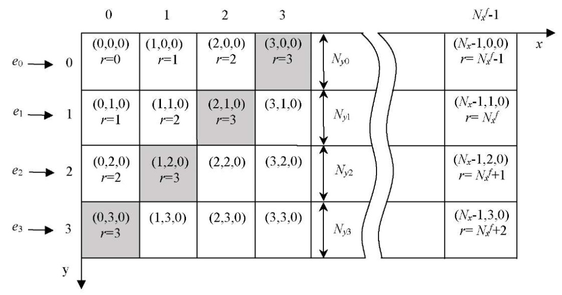
Fig. 1. Parallel-pipelined computing process
Research Results. The computational experiments were carried out on K-60 high-performance computing system of the Keldysh Applied Mathematics Institute, RAS. A GPU section was used, each node of which was equipped with two Intel Xeon Gold 6142 v4 processors, four Nvidia Volta GV100GL video adapters and 768 GB of RAM.
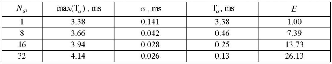
The computational experiment consisted of two stages — preparatory and basic. At the preparatory stage, the correctness of the decomposition of the computational domain into subsections, blocks and fragments was checked by step-by-step comparison of values in the nodes of the initial grid and in fragments obtained as a result of decomposition. Then, the operation of the flow control algorithm during which the time spent on calculating 1, 8, 16 and 32 fragments of the computational grid with a dimension of 50 nodes by spatial coordinates  ,
,  ,
,  , and the same number of CPU streams
  was checked by the iterative alternating-triangular method in parallel mode. Ten repetitions were performed with the calculation of the arithmetic mean
  and standard deviation
  . Based on the data obtained, time
  spent by each stream on processing one fragment of the computational grid and acceleration
  , equal to the ratio of the processing time
  of one fragment
  by streams to the corresponding processing time by one stream
  was calculated. The experimental data are given in Table 1. The experiment showed that the standard deviation had the smallest value in the case of using 32 parallel CPU streams and was 0.026 ms, i.e., using 32 parallel CPU streams when calculating 32 fragments of the computational grid gave a more uniform time load of program streams, which generally increased the efficiency of the computing node. At the same time, the average value of the calculation of one fragment was 4.14 ms. The dependence of acceleration on the number of streams turned out to be linear
  , with a coefficient of determination equal to 0.99. We have found that with an increase in the number of streams, the acceleration of the developed algorithm increases. This indicates the efficient use of the subsystem when working with memory.
Table 1
Results of the preparatory stage of the computational experiment
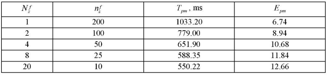
At the basic stage of the computational experiment, a three-dimensional computational domain having dimensions of 1,600; 1,600; 200 by spatial coordinates  ,
,  and
and  , accordingly, was divided into 32 fragments of 50 nodes for each of the coordinates
  and
and  . The division into fragments by coordinate
  is given in Table 2. For each decomposition option with a tenfold repetition, the processing time of the entire computational grid was measured by the proposed parallel-conveyor method, and its average value
  was calculated. Acceleration
  was calculated as ratio
  to time
  of the calculation by sequential version of the algorithm, equal to 6.963 ms. Regression equation
  with a determination coefficient equal to 0.94 was obtained. Analysis of the results of the basic stage of the computational experiment showed a significant slowdown in growth
  at
at  . Therefore, we conclude that splitting into fragments by coordinate
  by an amount not exceeding 10 is optimal.
Table 2
Results of the main stage of the computational experiment
Discussion and Conclusion. As a result of the conducted research, a model of a parallel-pipeline computing process was developed by the example of one of the most intensive stages of solving a system of grid equations by a modified alternating-triangular iterative method. Its construction was based on decomposition models of a three-dimensional uniform computational grid, taking into account the technical characteristics of the equipment used in the calculations.
The results obtained under the computational experiments validated the effectiveness of the developed method. The correctness of the decomposition of the computational domain into subsections, blocks and fragments was also confirmed. The operation of the flow control algorithm was verified. At the same time, it was revealed that the standard deviation had the smallest value in the case of using 32 parallel CPU streams and is 0.026 ms, i.e., using 32 parallel CPU streams when calculating 32 fragments of the computational grid gave a more uniform time load of program streams. Here, the average value of the calculation of one fragment was 4.14 ms.
The results of processing the measurements of the calculation time by the proposed parallel-conveyor method showed a significant slowdown in the growth of acceleration when divided into fragments by coordinate  at
at  . It was found that splitting into fragments by coordinate
  by an amount not exceeding 10 was optimal.
1. Shiganova TA, Alekseenko E, Kazmin AS. Predicting Range Expansion of Invasive Ctenophore Mnemiopsis leidyi A. Agassiz 1865 under Current Environmental Conditions and Future Climate Change Scenarios. Estuarine, Coastal and Shelf Science. 2019;227:106347. https://doi.org/10.1016/j.ecss.2019.106347
2. Sukhinov AI, Chistyakov AE, Nikitina AV, Filina AA, Lyashchenko TV, Litvinov VN. The Use of Supercomputer Technologies for Predictive Modeling of Pollutant Transport in Boundary Layers of the Atmosphere and Water Bodies. In book: L Sokolinsky, M Zymbler (eds). Parallel Computational Technologies. Cham: Springer; 2019. P. 225–241. 10.1007/978-3-030-28163-2_16
3. Rodriguez D, Gomez D, Alvarez D, Rivera S. A Review of Parallel Heterogeneous Computing Algorithms in Power Systems. Algorithms. 2021;14(10):275. 10.3390/a14100275.
4. Abdelrahman AM Osman. GPU Computing Taxonomy. In ebook: Wen-Jyi Hwang (ed). Recent Progress in Parallel and Distributed Computing. London: InTech; 2017. http://dx.doi.org/10.5772/intechopen.68179
5. Parker A. GPU Computing: The Future of Computing. In: Proceedings of the West Virginia Academy of Science. Morgantown, WV: WVAS; 2018. Vol. 90 (1). 10.55632/pwvas.v90i1.393
6. Nakano Koji. Theoretical Parallel Computing Models for GPU Computing. In book: Koç Ç. (ed). Open Problems in Mathematics and Computational Science. Cham: Springer; 2014. P. 341–359. 10.1007/978-3-319-10683-0_14
7. Bhargavi K, Sathish Babu B. GPU Computation and Platforms. In book: Ganesh Chandra Deka (ed). Emerging Research Surrounding Power Consumption and Performance Issues in Utility Computing. Hershey, PA: IGI Global; 2016. P.136–174. 10.4018/978-1-4666-8853-7.ch007
8. Ebrahim Zarei Zefreh, Leili Mohammad Khanli, Shahriar Lotfi, Jaber Karimpour. 3 Level Perfectly Nested Loops on Heterogeneous Distributed System. Concurrency and Computation: Practice and Experience. 2017;29(5):e3976. 10.1002/cpe.3976
9. Fan Yang, Tongnian Shi, Han Chu, Kun Wang. The Design and Implementation of Parallel Algorithm Accelerator Based on CPU-GPU Collaborative Computing Environment. Advanced Materials Research. 2012;529:408–412. 10.4028/www.scientific.net/AMR.529.408
10. Varshini Subhash, Karran Pandey, Vijay Natarajan. A GPU Parallel Algorithm for Computing Morse-Smale Complexes. IEEE Transactions on Visualization and Computer Graphics. 2022. P. 1–15. 10.1109/TVCG.2022.3174769
11. Leiming Yu, Fanny Nina-Paravecino, David R Kaeli, Qianqian Fang. Scalable and Massively Parallel Monte Carlo Photon Transport Simulations for Heterogeneous Computing Platforms. Journal of Biomedical Optics. 2018;23(1):010504. 10.1117/1.JBO.23.1.010504
12. Fujimoto RM. Research Challenges in Parallel and Distributed Simulation. ACM Transactions on Modeling and Computer Simulation. 2016;26(4):1–29. 10.1145/2866577
13. Qiang Qin, ChangZhen Hu, TianBao Ma. Study on Complicated Solid Modeling and Cartesian Grid Generation Method. Science China Technological Sciences. 2014;57:630–636. 10.1007/s11431-014-5485-5
14. Seyong Lee, Jeffrey Vetter. Moving Heterogeneous GPU Computing into the Mainstream with Directive-Based, High-Level Programming Models. In: Proc. DOE Exascale Research Conference. Portland, Or; 2012.
15. Thoman P, Dichev K, Heller Th, Iakymchuk R, Aguilar X, Hasanov Kh, et al. A Taxonomy of Task-Based Parallel Programming Technologies for High-Performance Computing. Journal of Supercomputing. 2018;74(2):1422– 1434. 10.1007/s11227-018-2238-4
Vladimir N. Litvinov, Cand.Sci. (Eng.), Associate Professor of the Mathematics and Informatics
1, Gagarin sq., Rostov-on-Don, 344003
Nelli B. Rudenko, Cand.Sci. (Eng.), Associate Professor, Associate Professor of the Mathematics and Bioinformatics Department
21, Lenina St., Zernograd, 347740
Natalya N. Gracheva, Cand.Sci. (Eng.), Associate Professor of the Mathematics and Bioinformatics Department
21, Lenina St., Zernograd, 347740
Litvinov V.N., Rudenko N.B., Gracheva N.N. Model of a Parallel-Pipeline Computational Process for Solving a System of Grid Equations. Advanced Engineering Research (Rostov-on-Don). 2023;23(3):329-339. https://doi.org/10.23947/2687-1653-2023-23-3-329-339


Advanced Engineering Research (Rostov-on-Don)
ISSN 2687-1653 (Online)
Contact with: Publisher / Editorial Office of the Journal
Publisher: Don State Technical University - DSTU, Rostov-on-Don, Russia - https://donstu.ru/en/
Editor-in-Chief: Alexey N. Beskopylny, Dr.Sci. (Eng.), Professor, Vice-Rector, Don State Technical University (Rostov-on-Don, Russia)
Don State Technical University
1, Gagarin Sq., Rostov-on-Don, 344003, Russia
tel.: +7 (863) 2738-372, e-mail: vestnik@donstu.ru
16+
Processing of personal data