Contents
Scroll to:
https://doi.org/10.23947/2687-1653-2024-24-1-36-47
EDN: HTOURY
Scroll to:
Introduction. All polymer materials and composites based on them are characterized by pronounced rheological properties, the prediction of which is one of the most critical tasks of polymer mechanics. Machine learning methods open up great opportunities in predicting the rheological parameters of polymers. Previously, studies were conducted on the construction of predictive models using artificial neural networks and the CatBoost algorithm. Along with these methods, due to the capability to process data with highly nonlinear dependences between features, machine learning methods such as the k-nearest neighbor method, and the support vector machine (SVM) method, are widely used in related areas. However, these methods have not been applied to the problem discussed in this article before. The objective of the research was to develop a predictive model for evaluating the rheological parameters of polymers using artificial intelligence methods by the example of polyvinyl chloride.
Materials and Methods. This paper used k-nearest neighbor method and the support vector machine to determine the rheological parameters of polymers based on stress relaxation curves. The models were trained on synthetic data generated from theoretical relaxation curves constructed using the nonlinear Maxwell-Gurevich equation. The input parameters of the models were the amount of deformation at which the experiment was performed, the initial stress, the stress at the end of the relaxation process, the relaxation time, and the conditional end time of the process. The output parameters included velocity modulus and initial relaxation viscosity coefficient. The models were developed in the Jupyter Notebook environment in Python.
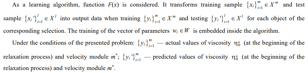
Results. New predictive models were built to determine the rheological parameters of polymers based on artificial intelligence methods. The proposed models provided high quality prediction. The model quality metrics in the SVR algorithm were: MAE – 1.67 and 0.72; MSE – 5.75 and 1.21; RMSE – 1.67 and 1.1; MAPE – 8.92 and 7.3 for the parameters of the initial relaxation viscosity and velocity modulus, respectively, with the coefficient of determination R2 – 0.98. The developed models showed an average absolute percentage error in the range of 5.9 – 8.9%. In addition to synthetic data, the developed models were also tested on real experimental data for polyvinyl chloride in the temperature range from 20° to 60°C.
Discussion and Conclusion. The approbation of the developed models on real experimental curves showed a high quality of their approximation, comparable to other methods. Thus, the k-nearest neighbor algorithm and SVM can be used to predict the rheological parameters of polymers as an alternative to artificial neural networks and the CatBoost algorithm, requiring less effort to preset adjustment. At the same time, in this research, the SVM method turned out to be the most preferred method of machine learning, since it is more effective in processing a large number of features
Kondratieva T.N., Chepurnenko A.S. Prediction of Rheological Parameters of Polymers by Machine Learning Methods. Advanced Engineering Research (Rostov-on-Don). 2024;24(1):36-47. https://doi.org/10.23947/2687-1653-2024-24-1-36-47. EDN: HTOURY
Introduction. Polymers are used in various industries, including the production of plastics, textiles, packaging materials, and more. Accurate prediction of the rheological parameters of polymers is a complex task that is important for optimizing production processes and creating products with desired properties.
Today, machine learning methods have gained great popularity in various fields, including chemistry and materials science, due to their ability to efficiently process and analyze large amounts of data. These methods make it possible to predict the properties of materials. In [1], a platform based on machine learning was described, and the integration of metrological support in the context of digital transformation was proposed. In [2], the local distribution of deformation, the development of plastic anisotropy, and fracture in additively manufactured alloys were predicted. The problems of developing measuring control regulators on digital platforms were formulated in [3]. An intelligent model for controlling the parameters of overlap joint welding was built in [4]. However, the issues of using machine learning methods to predict the rheological properties of polymers remain insufficiently investigated. This is caused by both technical and methodological difficulties, such as the heterogeneity of the polymer structure, their sensitivity to external conditions, and complex interactions between molecules during deformation.
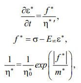
Research in the field of rheological properties of polymers and composites using machine learning methods has great prospects in the construction industry [5]. For numerous polymers, the experimental data are well described by the generalized nonlinear Maxwell-Gurevich equation [6], which has the form for a uniaxial stress state [7]:
 (1)
(1)
where ε* — creep deformation, f* — stress function, σ — stress, E∞ — module of high elasticity,  — initial relaxation viscosity, m* — velocity module.
Various intelligent machine learning models can be used to determine the rheological parameters of polymers, such as the initial relaxation viscosity (hereinafter just “viscosity”) and the velocity module [8, 9]. For example, one such model is a neural network that can be trained on generated datasets to determine optimal polymer parameters [10].
Prediction based on synthesized data is a fairly common practice, including for nonlinear optimization
methods [11, 12]. One of the ways to generate data is the use of Rosenbrock, Himmelblau, and Booth functions [13], which are effectively applied to test optimization methods such as gradient descent methods, genetic algorithms, and the Newton method. This approach was applied in [14], where a data set based on theoretical stress relaxation curves using the nonlinear Maxwell-Gurevich equation was generated to test the efficiency of various optimization methods.
In [15], several machine learning approaches were given to predict the durability of a reinforced concrete beam, such as a neural network of back propagation, linear and ridge regression, a decision tree, and a random forest. The input parameters of the study were both various characteristics of the material and their properties, depending on the environment (temperature, humidity). Finally, according to the results of the study, the back propagation model determined a more accurate forecast (85%), the average values (MAE) and MAPE were 1.13% and 14.5%, respectively.
Another approach to solving inverse problems of creep theory using the neural network method is based on training a model on large amounts of experimental data. In [16], a neural network model was developed, which was trained on data obtained as a result of long-term experiments on polymer materials, and successfully predicted the viscoelastic behavior of these materials. The data obtained from experiments on samples of various materials were used for the study.
Unlike the above-mentioned papers, the presented research is intended to promote the development of more accurate and reliable methods for predicting polymer properties, such as the k-nearest neighbor method and the support vector machine, which is important for various industries and science.
The research objective was to develop a predictive model based on artificial intelligence methods for analyzing the rheological properties of polymers. Previously, the authors had already used a machine learning algorithm based on gradient boosting CatBoost to process stress relaxation curves [17, 18]. CatBoost is one of the most powerful machine learning algorithms applicable to solving not only regression problems, but also classification and ranking problems [19].
The CatBoost method can be useful for solving some tasks, but it also has its limitations and disadvantages. In this regard, there is an interest in using other algorithms mentioned earlier [20] to solve the problem.
Materials and Methods. The generated data array is partially presented in Table 1. This array was formed on the basis of theoretical stress relaxation curves described by the Maxwell-Gurevich equation, according to the technique presented in [14]. The variation ranges of the velocity modulus and the initial relaxation viscosity in the generated array correspond to the real ranges for polyvinyl chloride in the temperature interval from 20° to 60°C. The total number of numerical experiments (n) was 30,000.
Table 1
Table of initial data for training the model
|
No |
Deformation, % |
Stress at the beginning of the process σ0, MPa |
Stress at the end of the process σ∞, MPa |
Relaxation time tn, h |
Conditional end time of the process t95, h |
Velocity module m*, MPa |
Viscosity 106, MPa∙s |
|
1 |
1.000 |
10.000 |
0.909 |
0.277 |
1.484 |
6.000 |
3.000 |
|
2 |
2.000 |
20.000 |
1.818 |
0.109 |
1.003 |
6.000 |
3.000 |
|
3 |
3.000 |
30.000 |
2.727 |
0.046 |
0.820 |
6.000 |
3.000 |
|
4 |
1.000 |
10.000 |
0.909 |
0.861 |
4.615 |
6.000 |
9.333 |
|
5 |
2.000 |
20.000 |
1.818 |
0.339 |
3.122 |
6.000 |
9.333 |
|
6 |
3.000 |
30.000 |
2.727 |
0.142 |
2.552 |
6.000 |
9.333 |
|
7 |
1.000 |
10.000 |
0.909 |
1.445 |
7.747 |
6.000 |
15.667 |
|
… |
|||||||
|
29997 |
3 |
45 |
37.5 |
0.285 |
2.476 |
15 |
53.666 |
|
29998 |
1 |
15 |
12.5 |
1.003 |
4.255 |
15 |
60 |
|
29999 |
2 |
30 |
25 |
0.558 |
3.371 |
15 |
60 |
|
30000 |
3 |
45 |
37.5 |
0.319 |
2.769 |
15 |
60 |
The data set consisted of five input variables and two output variables. Input variables (unit measure):
deformation — ε (%); stress at the beginning of the process — σ0 (MPa); stress at the end of the process — σ∞ (MPa); relaxation time — tn (h); conditional end time of the process — t95 (h). Output variables (unit measure): velocity
module — m* (MPa); initial relaxation viscosity —  (in Table 1 and further, simply “viscosity”) (106 MPa∙s).
Values σ0, σ∞, tn и t95 are schematically shown on the typical stress relaxation curve (Fig. 1).
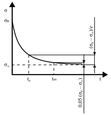
Fig. 1. Typical stress relaxation curve
The k-nearest neighbor (k-NN) algorithm is based on the similarity analysis of nearby objects. The k-NN method is in great demand for solving various types of machine learning tasks.
Formula (2) represents the general form of the algorithm, where w(i, x) — weight function evaluating the importance of the i-th neighbor.
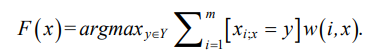 (2)
(2)
The maximum total weight can be achieved for several objects at the same time. The entropy of this process can be adjusted using nonlinear sequence w(i, x) = [i ≤ k]qi (exponentially weighted k-nearest neighbor method) provided that 0 ≤ q ≤ 0.5.
Representing a fairly simple machine learning algorithm, k-NN is well applicable to solving classification and regression problems. The advantages of this method are ease of implementation, no need for pre-training of the model. It is used for all types of data, including categorical and numeric. Disadvantages: a tendency to over-training (provided that k is too small), poor performance with large amounts of data, it is not possible to take into account the relationship between the signs.
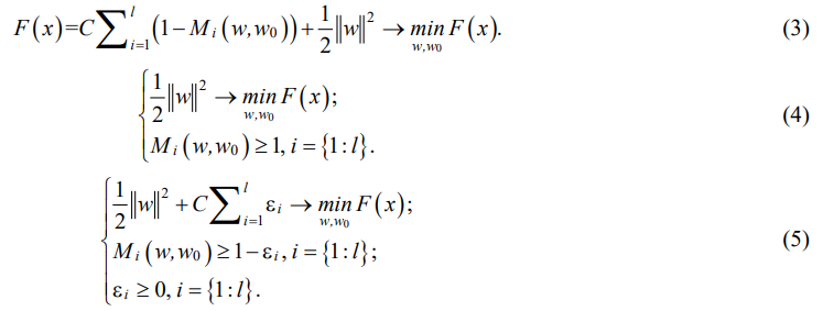
The support vector algorithm — support vector regression (SVR) — solves the problem of minimizing the sum of the mean absolute error. SVR is more resistant to outliers, unlike the least squares method, due to the regularization coefficient (C) and the “epsilon-insensitive tube” (ε). In this case, ε determines the width of the tube in which errors are ignored. Stochastic gradient descent is used to find the minimum of the function.
The support vector machine learning algorithm is function F(x) of approximation and regularization of empirical risk, which converts training and test samples into output data for each object of the corresponding sample. Formula (3) represents the general form of the algorithm, (4) is a linearly separable sample, (5) is a linearly inseparable sample, where C — regularization coefficient, Mi(w, w0) — scalar product of vectors (feature and support vector), wi— weight coefficients.
Function  is a function of a pair of objects
  , п representable as a scalar product in some space H, for which transformation
  takes place. Function
  — kernel if
  , provided that K is symmetric:
  and nonnegative definite:
 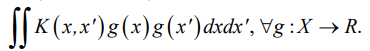 The regularization coefficient is determined by the sliding mode control method.
Advantages of the SVM method are as follows: high accuracy in classification problems in nonlinear spaces; ability to work with a large number of features (including categorical and numerical), generalize data (which provides applying the model to new data), work with data that are not linearly separable due to the use of kernel functions.
Disadvantages of the SVM method include inefficiency of working with large amounts of data; low interpretability of the model; the requirement to configure numerous parameters, such as the type of kernel (its parameters, regularization parameters), etc.
In this research, algorithms are developed in the Jupyter Notebook intelligent computing environment using machine learning methods.
The selection of such a parameter as the number of neighbors affects the generalizing ability of the developed model and is important for its correct operation. The most suitable algorithm for calculating distance based on data is Distance, in which the weights of objects are inversely proportional to their distance. Accordingly, in the case of closer neighbors of the query object, they have more influence than their neighbors located at a greater distance from the object.
The data set was divided into training and test samples in a ratio of 75/25. In turn, 20% of the training sample became validation. The sample size was: training — xtrain = 20,400; test — xtest = 6,000; validation — xeval = 3,600. For variables ytrain, ytest, yeval, the data were distributed in a similar way.
To build the k-nearest neighbor model, the following parameters were selected: number of neighbors, sheet size, interval, and weight function. The range and functionality of the values for the configurable parameters are shown in Table 2.
Table 2
Parameter table for k-NN model
|
No |
Parameter |
Value |
Functional |
|
1 |
Number of neighbors (k) |
3, 5, 7, 9 |
Determines optimal number of neighbors for query |
|
2 |
Sheet size (n) |
15, 20, 30 |
Determines speed of querying and required memory for storing the tree |
|
3 |
Interval (p) |
1 (l1), 2 (l2) |
Defines power parameter (Minkowski metric) |
|
4 |
Weight function (w) |
'uniform', 'distance' |
Predicting weights |
To build the SVR model, the following parameters were selected: kernel type, kernel order, regularization coefficient (quadratic regularizer), ε. The range and functional values for the adjustable parameters are presented in Table 3.
Table 3
Parameter table for SVR model
|
No |
Parameter |
Value |
Functional |
|
1 |
Kernel type |
'linear'; 'poly'; 'rbf'; 'sigmoid' |
Defines type of hyperplane (linear/nonlinear) |
|
2 |
Kernel order |
1, 2, 3, 4, 5, 7 |
Defines degree of polynomial function of kernel |
|
3 |
Quadratic regularizer (C) |
2; 3; 4; 5; 7; 10 |
Solves problems of vector multicollinearity |
|
4 |
ε |
0.1; 0.2; 0.5; 1; 1.5; 2; 3 |
Determines deviation of the object (proximity measure) |
Figure 2 shows the correlations between the variables.
The following types of linear correlations between individual input and output variables of the model can be noted:
 “Relaxation time” and “End time of the process”
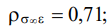 “Stress at the beginning” and “Stress at the end”
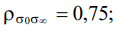
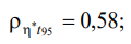 “Viscosity” and “Relaxation time”
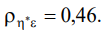
The presence of a moderate correlation between variables or its absence indicates only the absence of a linear relationship; therefore, it is possible to have a nonlinear relationship between variables.
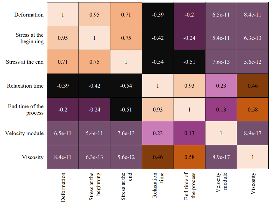
Fig. 2. Correlation matrix
Table 4 shows the statistical characteristics of the original data set.
Table 4
Statistical characteristics of the original data set
|
Parameter |
ε |
σ0 |
σ∞ |
tn |
t95 |
m* |
|
|
Unit measure |
% |
MPa |
MPa |
h |
h |
MPa |
106 MPa∙s |
|
count |
30,000.00 |
30,000.00 |
30,000.00 |
30,000.00 |
30,000.00 |
30,000.00 |
30,000.00 |
|
mean |
2.00 |
25.00 |
15.78 |
0.75 |
4.41 |
10.50 |
31.50 |
|
std |
0.82 |
10.77 |
9.10 |
0.94 |
4.40 |
2.87 |
18.19 |
|
min |
1.00 |
10.00 |
0.91 |
0.00 |
0.07 |
6.00 |
3.00 |
|
max |
3.00 |
45.00 |
37.50 |
10.04 |
38.02 |
15.00 |
60.00 |
The best parameters for the k-nearest neighbor model were determined as a result of 5-block cross-validation (Table 5).
Table 5
Best k-NN model parameters
|
Parameter |
Number of neighbors (k) |
Sheet size (n) |
Interval (p) |
Weight function (w) |
|
3 |
15 |
2 |
'distance' |
|
m* |
5 |
15 |
2 |
'distance' |
The best parameters of the SVR model for viscosity parameters (at the beginning of the relaxation process) and velocity module were obtained empirically (Table 6).
Table 6
Best parameters of SVR model
|
Parameter |
Kernel type |
Kernel order |
Quadratic regularizer |
ε |
|
'rbf' |
2 |
5 |
0.3 |
|
m* |
'rbf' |
3 |
6 |
0.3 |
The ratio between the real and predicted values for the k-NN model in terms of the parameters “Viscosity” and “Velocity modulus” is shown in Figures 3, 4.
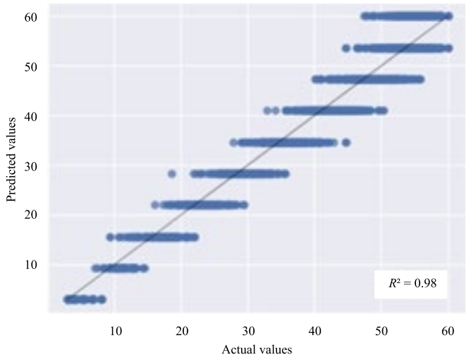
Fig. 3. Diagrams of prediction errors of k-NN, “Viscosity”
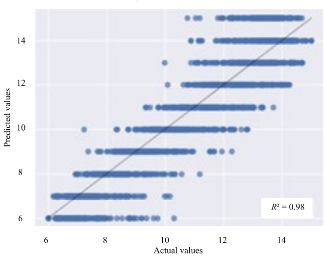
Fig. 4. Diagrams of prediction errors of k-NN, “Velocity module”
The ratio between the real and predicted values for the SVR model according to the parameters “Viscosity” and “Velocity module” is shown in Figures 5, 6.
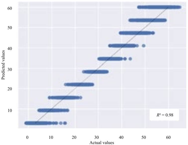
Fig. 5. Diagrams of prediction errors of k-NN, “Viscosity”
![]()
Fig. 6. Diagrams of prediction errors of k-NN, “Velocity module”
The metrics of the developed models of k-nearest neighbors and support vectors are presented in Tables 7 and 8, respectively.
Table 7
Metrics of the developed k-NN models
|
Parameter |
MAE |
MSE |
RMSE |
MAPE (%) |
R2 train |
R2 test |
| |
1.8 |
6.8 |
2.6 |
5.9 |
1.00 |
0.98 |
|
m* |
0.7 |
0.8 |
0.9 |
6.9 |
0.99 |
0.98 |
Table 8
Metrics of the developed SVR models
|
Parameter |
MAE |
MSE |
RMSE |
MAPE (%) |
R2 train |
R2 test |
| |
1.67 |
5.75 |
1.67 |
8.92 |
0.98 |
0.97 |
|
m* |
0.72 |
1.21 |
1.1 |
7.3 |
0.89 |
0.87 |
In addition to synthetic data, the developed models were also tested on real experimental data presented in [13]. Experimental relaxation curves of polyvinyl chloride were used for various temperatures in the range from 20° to 60°C. In Figure 7, the experimental stress values at different temperatures at different points in time are marked with felt-tip pens, and solid lines show stress relaxation curves based on values m* and predicted by the models.
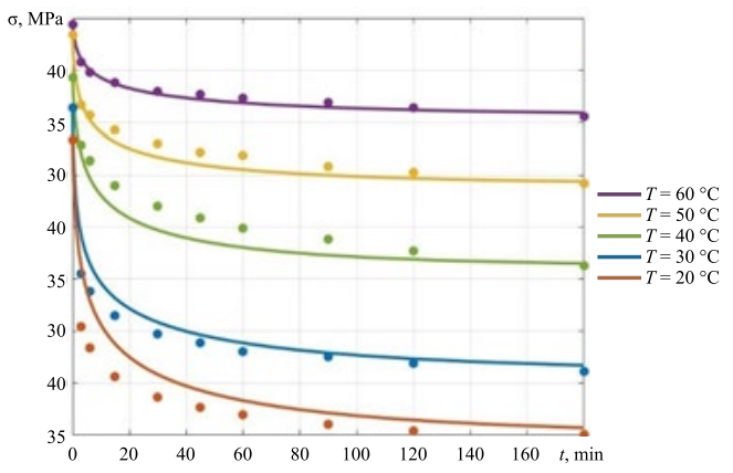
Fig. 7. Results of testing the model on experimental data
Discussion and Conclusion. Figure 5 shows that the quality of prediction based on experimental data is quite high, specifically, for temperatures of 30°C, 50°C and 60°C. For other temperatures, the prediction quality is somewhat lower, which is due to the quality of the experimental curves themselves. It was necessary to extend the experiment time and wait for the curves to reach the horizontal asymptote.
In this research, the most preferred method is the support vector machine (SVM). This is due to the fact that SVM can process data with a large number of features, which is important for the analysis of rheological parameters of materials. In addition, SVM works with nonlinear dependences between features, it is applicable to solve the regression problem, which is required to determine the rheological parameters of materials.
However, the CatBoost method can also be effective in this task, especially, if there are categorical features in the data. In addition, CatBoost can process missing data, which can be important for analyzing rheological parameters of materials.
The k-nearest neighbor method is less preferable in this task due to its low efficiency in processing a large number of features, as well as the presence of problems with high data dimensionality.
In the course of the investigation, it has been shown that the use of machine learning methods makes it possible to effectively analyze and process large amounts of data, including information about the characteristics of polymers and their rheological properties. The model developed on the basis of such an analysis maintains high accuracy in predicting the rheological parameters of polyvinyl chloride, which is confirmed by the results of cross-validation and comparison to experimental data.
One of the key advantages of this approach is the ability to automate the process of predicting the rheological parameters of polymers, which reduces the time and cost of research and development of new materials. In addition, the model can be easily adapted to analyze other types of polymers and predict their properties.
As a result of this research, a predictive model has been developed to evaluate the rheological parameters of polyvinyl chloride using artificial intelligence methods based on data of its characteristics and rheological properties. The model demonstrates high prediction accuracy and can be used to optimize the production and development of new polymer-based materials.
1. Dudukalov EV, Munister VD, Zolkin AL, Losev AN, Knishov AV. The Use of Artificial Intelligence and Information Technology for Measurements in Mechanical Engineering and in Process Automation Systems in Industry 4.0. Journal of Physics: Conference Series. IOP Publishing. 2021;1889(5):052011. https://doi.org/10.1088/1742-6596/1889/5/052011
2. Waqas Muhammad, Abhijit P Brahme, Olga Ibragimova, Jidong Kang, Kaan Inal. A Machine Learning Framework to Predict Local Strain Distribution and the Evolution of Plastic Anisotropy & Fracture in Additively Manufactured Alloys. International Journal of Plasticity. 2021;136:102867. https://doi.org/10.1016/j.ijplas.2020.102867
3. Won-Bin Oha, Tae-Jong Yuna, Bo-Ram Leea, Chang-Gon Kima, Zong-Liang Lianga, Ill-Soo Kim. A Study on Intelligent Algorithm to Control Welding Parameters for Lap-joint. Procedia Manufacturing. 2019;30:48–55. http://doi.org/10.1016/j.promfg.2019.02.008
4. Amit R Patel, Kashyap K Ramaiya, Chandrakant V Bhatia, Hetalkumar N Shah, Sanket N Bhavsar. Artificial Intelligence: Prospect in Mechanical Engineering Field—A Review. In book: Data Science and Intelligent Applications. Singapore: Springer; 2021. P. 267–282. https://doi.org/10.1007/978-981-15-4474-3_31
5. Amjadi M, Fatemi A. Creep and Fatigue Behaviors of High-Density Polyethylene (HDPE): Effects of Temperature, Mean Stress, Frequency, and Processing Technique. International Journal of Fatigue. 2020;141:105871. http://doi.org/10.1016/j.ijfatigue.2020.105871
6. Chepurnenko V, Yazyev B, Xuanzhen Song. Creep Calculation for a Three-Layer Beam with a Lightweight Filler. MATEC Web of Conferences. 2017;129:05009. https://doi.org/10.1051/matecconf/201712905009
7. Litvinov SV, Yazyev BM, Turko MS. Effecting of Modified HDPE Composition on the Stress-Strain State of Constructions. IOP Conference Series: Materials Science and Engineering. 2018;463(4):042063. https://doi.org/10.1088/1757-899X/463/4/042063
8. Guangjian Xiang, Deshun Yin, Ruifan Meng, Siyu Lu. Creep Model for Natural Fiber Polymer Composites (NFPCs) Based on Variable Order Fractional Derivatives: Simulation and Parameter Study. Journal of Applied Polymer Science. 2020;137(24):48796. http://doi.org/10.1002/app.48796
9. Tugce Tezel, Volkan Kovan, Eyup Sabri Topal. Effects of the Printing Parameters on Short‐Term Creep Behaviors of Three‐Dimensional Printed Polymers. Journal of Applied Polymer Science. 2019;136(21):47564. http://doi.org/10.1002/app.47564
10. Litvinov SV, Trush LI, Yazyev SB. Flat Axisymmetrical Problem of Thermal Creepage for Thick-Walled Cylinder Made of Recyclable PVC. Procedia Engineering. 2016;150:1686–1693. https://doi.org/10.1016/j.proeng.2016.07.156
11. Dudnik AE, Chepurnenko AS, Litvinov SV. Determining the Rheological Parameters of Polyvinyl Chloride, with Change in Temperature Taken into Account. International Polymer Science and Technology. 2017;44(1):43–48. https://doi.org/10.1177/0307174X1704400109
12. Litvinov S, Yazyev S, Chepurnenko A, Yazyev B. Determination of Rheological Parameters of Polymer Materials Using Nonlinear Optimization Methods. In book: A. Mottaeva (ed). Proceedings of the XIII International Scientific Conference on Architecture and Construction. Singapore: Springer; 2020. P. 587–594. https://doi.org/10.1007/978-981-33-6208-6_58
13. Solovyova EB, Askadskiy AA, Popova MN. Investigation of Relaxation Properties of Primary and Secondary Polyvinyl Chloride. Plasticheskie massy. 2013;2:54–62. (In Russ.).
14. Chepurnenko A. Determining the Rheological Parameters of Polymers Using Artificial Neural Networks. Polymers. 2022;14(19):3977. https://doi.org/10.3390/polym14193977
15. Yu Xuan Rui. Developing an Artificial Neural Network Model to Predict the Durability of the RC Beam by Machine Learning Approaches. Case Studies in Construction Materials. 2022;17:e01382. http://doi.org/10.1016/j.cscm.2022.e01382
16. Nagababu Andraju, Greg W Curtzwiler, Yun Ji, Kozliak Evguenii, Prakash Ranganathan. Machine-Learning-Based Predictions of Polymer and Postconsumer Recycled Polymer Properties. A Comprehensive Review. ACS Applied Materials & Interfaces. 2022;14(38):42771–42790. http://doi.org/10.1021/acsami.2c08301
17. Chepurnenko AS, Kondratieva TN, Deberdeev TR, Akopyan VF, Avakov AA, Chepurnenko VS. Prediction of Rheological Parameters of Polymers Using CatBoost Gradient Boosting Algorithm. All Materials: Encyclopedic Reference Book. 2023;(6):21–29. (In Russ.).
18. Kondratieva T, Prianishnikova L, Razveeva I. Machine Learning for Algorithmic Trading. E3S Web of Conferences. 2020;224:01019. https://doi.org/10.1051/e3sconf/202022401019
19. Stelmakh SA, Shcherban EM, Beskopylny AN, Mailyan LR, Meskhi B, Razveeva I, et al. Prediction of Mechanical Properties of Highly Functional Lightweight Fiber-Reinforced Concrete Based on Deep Neural Network and Ensemble Regression Trees Methods. Materials. 2022;15(19):6740. https://doi.org/10.3390/ma15196740
20. Beskopylny AN, Stelmakh SA, Shcherban EM, Mailyan LR, Meskhi B, Razveeva I, et al. Concrete Strength Prediction Using Machine Learning Methods CatBoost, k-Nearest Neighbors, Support Vector Regression. Applied Sciences. 2022;12(21):10864. https://doi.org/10.3390/app122110864
Tatiana N. Kondratieva, Cand.Sci. (Eng.), Associate Professor of the Mathematics and Informatics Department
1, Gagarin sq., Rostov-on-Don, 344003
Anton S. Chepurnenko, Dr.Sci. (Eng.), Associate Professor, professor of the Strength of Materials Department
1, Gagarin sq., Rostov-on-Don, 344003
Kondratieva T.N., Chepurnenko A.S. Prediction of Rheological Parameters of Polymers by Machine Learning Methods. Advanced Engineering Research (Rostov-on-Don). 2024;24(1):36-47. https://doi.org/10.23947/2687-1653-2024-24-1-36-47. EDN: HTOURY


Advanced Engineering Research (Rostov-on-Don)
ISSN 2687-1653 (Online)
Contact with: Publisher / Editorial Office of the Journal
Publisher: Don State Technical University - DSTU, Rostov-on-Don, Russia - https://donstu.ru/en/
Editor-in-Chief: Alexey N. Beskopylny, Dr.Sci. (Eng.), Professor, Vice-Rector, Don State Technical University (Rostov-on-Don, Russia)
Don State Technical University
1, Gagarin Sq., Rostov-on-Don, 344003, Russia
tel.: +7 (863) 2738-372, e-mail: vestnik@donstu.ru
16+
Processing of personal data