Contents
Scroll to:
https://doi.org/10.23947/2687-1653-2024-24-2-178-189
EDN: EYQXQZ
Scroll to:
Introduction. Computer modeling allows engineers to make valid design decisions by accurately assessing the thermal characteristics of design objects. The implementation of digital twin technology in the process of designing technical facilities is the current direction of scientific research and development. To do this, it is necessary to develop computer models whose accuracy meets the requirements for digital twins. However, the scientific literature does not widely present the results of research aimed at implementing digital twin technology in the design process. The general issues related to the use of digital twins in various industries are mainly considered. Therefore, the objective of this study was the development of a digital model and a comparative analysis of the accuracy of calculations of thermal characteristics of the design object.
Materials and Methods. The main tool for conducting the research was the methodology proposed by the authors for developing a computer model of thermal characteristics for the implementation of digital twin technology. The numerical solution was implemented through constructing a thermal model for calculating the temperature field based on the finite element method in the ANSYS engineering analysis system from ANSYS, Inc. (USA). For the analytical solution, a computer model of thermal characteristics developed on the basis of the state-space method, implemented in the ANSYS Twin Builder module, was used. The state-space model was matched to the behavior of the original thermal model through approximating the transfer function to the stepwise response of the thermal load using the time domain vector approximation method. Verification of the constructed analytical model was carried out in the engineering calculation system MATLAB from the MathWorks company (USA). The research was carried out for a 400V machine model manufactured by NPO “Stankostroenie” LLC, Sterlitamak (Russia).
Results. The developed digital model makes it possible to calculate the thermal characteristics of the design object with high accuracy. The results of the comparative analysis showed a high degree of correspondence between the values of thermal characteristics obtained using the proposed digital model and the results of numerical simulation. The maximum error in calculating thermal characteristics did not exceed 0.1ºC.
Discussion and Conclusion. Computer modeling that combines numerical calculation methods and a scientific approach based on digital twin technology, provides obtaining the result as close as possible to the results of experiments. The digital model proposed in the study is an effective solution, since it provides performing calculations to evaluate thermal characteristics in real time, which is one of the most important requirements for the implementation of digital twin technology.
Pozevalkin V.V., Polyakov A.N. Implementation of a Digital Model of Thermal Characteristics Based on the Temperature Field. Advanced Engineering Research (Rostov-on-Don). 2024;24(2):178-189. https://doi.org/10.23947/2687-1653-2024-24-2-178-189. EDN: EYQXQZ
Introduction. Computer modeling has traditionally been an effective tool for solving thermal problems at an early stage of designing complex technical facilities. However, solving the problem requires an accurate assessment of the thermal characteristics of the design object to reduce the negative effects caused by an increase in temperature [1]. At the same time, one of the effective tools for preliminary assessment of thermal characteristics is simulation modeling in an engineering analysis system based on advanced digital solutions and developments. In [2], for example, a developed digital twin for determining thermal characteristics was presented by the authors Jianying Xiao and Kangoo Fan. The principle of operation of the twin was to simulate the thermal behavior of an object through displaying and correcting thermal boundary conditions. The experimental results showed a high accuracy of the model (more than 95%), which was essential for improving the accuracy of modeling thermal characteristics and thermal optimization. Therefore, the urgent direction of scientific research and development in the field of modeling is the use of artificial intelligence systems [3] and digital twins [4]. In [3] by Haoran Yi and others, an interactive model for correcting thermal boundary conditions based on a neural network was proposed to improve the accuracy of the analysis of thermal characteristics. The experimental results showed that the accuracy of calculating the temperature field exceeded 98%, and the accuracy of predicting thermal deformation was 96%, which effectively increased the simulation accuracy. In addition, in [5] by Kurganova N.V. and others, it was noted that digital twins were often used to improve physical prototypes of complex technical objects, since they not only allow for the information support for the design process, but also contribute to effective design decisions based on developments in the field of artificial intelligence. One of the characteristic features of digital twin technology is that reduced-order computer models are often used for simulation [6]. Therefore, the development of computer models is one of the basic conditions for the implementation of digital twin technology [7]. Model order reduction is an effective and mathematically understandable approach to overcome the time constraints of multidimensional simulation models. In [8] by Mirzoev D.A. and others, for example, a simple analytical model of thermal fields was proposed for the development of digital counterparts of the industrial arc welding process. Bordachev E.V. and Lapshin V.P. [9] presented the results of mathematical modeling of the temperature in the tool–product contact zone under metal turning. This approach provides obtaining an accurate assessment of thermal characteristics corresponding to the results of numerical experiments in real time. Schröder C. and Matthias V. [10] presented a reduced-order model and proposed a new model balancing procedure based on the transformation of the state shift. In conclusion, they presented the results of a comparative analysis and the results from literature sources obtained through a series of numerical experiments. The use of a linear and time-invariant reduced-order computer model allows for fast simulation while maintaining high calculation accuracy [11]. When developing a computer model, approximation [12] of the transfer function is performed to approximate the state space model to the step response of the initial thermal model [13]. Since the step response of the thermal load is derived from the base thermal model, the digital model should provide the same values of thermal characteristics. However, despite the fact that recently there has been an increase in interest in the digital twin, the scientific literature does not widely present the results of research related to the implementation of digital solutions in the design of technical facilities. Based on a systematic review of the literature and thematic analysis of publications on digital twins, one of the key knowledge gaps associated with the development of mathematical, software and methodological support for high-precision computer models in the framework of the implementation of digital twin technology has been identified. In this regard, the objective of the study was to develop a reduced-order computer model and analyze its feasibility as part of a digital model for accurate calculation of thermal characteristics of complex technical design objects. To achieve that, it was necessary to build a thermal model and calculate the temperature field of the design object, generate independent step responses of the thermal load using the developed software scenario [14], implement a digital model for calculating thermal characteristics, determine the error of calculations obtained using numerical and analytical solutions, and conduct a comparative analysis of the simulation results.
Materials and Methods. The construction of the temperature field of the modeling object was performed for a homogeneous isotropic body on the basis of the equation of nonstationary thermal conductivity:
 (1)
(1)
where T — temperature (°C); t — time (s);  — diffusivity coefficient (m2/s); λ— thermal conductivity coefficient (W/m·°C); c — specific heat capacity (J/kg·°C); ρ — material density (kg/m3); ∆ — Laplace operator; qv — volumetric heat dissipation power (W/m3).
The heat flow in the heat transfer process was assumed to be equal to the amount of heat transferred through an arbitrary surface area S per unit time t. It is expressed by the following equation:
 (2)
(2)
where Q — heat flow (W); qn — heat-flux rate (W/m2); S — surface area (m2).
The density of the heat flux during heat transfer was determined from the formula:
 (3)
(3)
where α — heat transfer coefficient (W/(m2°C)); TS — surface temperature (°C); T∞ — ambient temperature (°C).
In this regard, to calculate the temperature field of the modeling object according to formula (1), heat flows (2) and (3) were set, which determined the amount of heat passing through the surface per unit time.
A component (Fig. 1) of a metal-cutting machine 400V model manufactured by NPO “Stankostroenie” LLC (Sterlitamak, Russia) in the form of a drillhead was selected as the object of modeling.
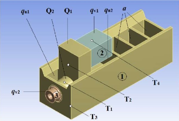
Fig. 1. Geometric model of the object in ANSYS Design Modeler:
1 — housing; 2 — electric motor; 3 — spindle assembly;
Q — heat flows; qv — volume heat release power;
qn — heat flux densities; a — heat transfer coefficient;
T1–T4 — temperature sensors
Since the amount of heat released mainly by the electric motor (electromagnetic losses) and the spindle assembly (mechanical friction losses) was taken into account for calculating the temperature field, electric motor qv1 and spindle assembly qv2, were taken as internal heat sources, near which the corresponding heat flows Q1 and Q2 were set. The densities of heat fluxes qn1, qn2 were assigned to surfaces located near the electric motor and spindle assembly, respectively.
Convection was determined by the heat transfer coefficient taking into account the conditions of heat transfer (natural convection in air). Since the machine is in contact with a gaseous medium (air), the amount of heat given by the heated surface to the environment per time unit t, is directly proportional to the difference in temperature between surface TS and medium T∞ depending on the area of the heat-emitting surface S (3).
When constructing a thermal model of an object (solid) consisting of a homogeneous material (structural steel) with constant thermophysical properties and the presence of internal heat sources, the following initial and boundary conditions were assigned:
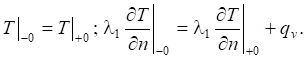 (4)
(4)
Heat flows (Q1, Q2), heat flux densities (qn1, qn2), as well as volume heat dissipation capacity (qv1, qv2), were assigned in accordance with well-known recommendations for metal-cutting machines [1]. Boundary conditions, as well as heat flows, were set for external surfaces. Therefore, it was taken into account that the interrelationships of thermal fields were present only between the outer surfaces.
Differential equation (1), together with the initial and boundary conditions of the second (2), third (3) and fourth (4) kinds, is a mathematical formulation of the problem. The task was solved using numerical and analytical modeling methods.
The numerical solution was performed on the basis of the finite element method in the ANSYS engineering analysis system, which is being developed by ANSYS Inc. (USA) and supplied by “Modeling and Digital Twins” AO, an authorized ANSYS distributor in Russia. The geometric model (Fig. 1) of the object was imported into the ANSYS Workbench project with the addition of the Transient Thermal analysis block. In the numerical solution, the simulation parameters and boundary conditions of the thermal model were calibrated (Table 1) to approximate the model temperature values to the experimental data.
Table 1
Boundary conditions (parameters) of the thermal model
|
Parameter |
Heat dissipation capacity |
Heat flows |
Heat flux densities |
Heat transfer coefficient |
|||
|
qv1, W/m³ |
qv2, W/m³ |
Q1, W |
Q2, W |
qn1, W/m² |
qn2, W/m² |
а, W/(m²·°С) |
|
|
Value |
6,500 |
1,000 |
28 |
15 |
32 |
18 |
15 |
In the ANSYS Mechanical module, the initial (initial temperature T0 = 24 °С) and boundary (Table 1) conditions were assigned for the developed grid model, the temperature field was constructed (Fig. 2). In this case, the thermal conductivity coefficient was assumed to be equal to λ = 60.5 W/(m·°С) and was assigned as such for structural steel.
The thermal model of the object included two contact connections for an electric motor and a spindle cartridge with a drillhead body, and contained 7 thermal boundary conditions. The developed grid model consisted of 16,309 elements and 58,527 nodes.
The total simulation time of 21,600 seconds (6 hours) was divided into intervals (1 hour) and steps ∆t = 360 seconds (6 minutes), a total of N = 60 steps within which the parameters of the thermal model (boundary conditions) were assumed to be constant and independent of time.
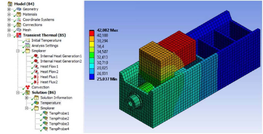
Fig. 2. Temperature field of the object in ANSYS Mechanical
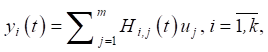
The calculation of the temperature field was required to generate an independent step response of the thermal load, containing information about temperature variation over time (thermal characteristics) for each parameter (Table 1) of the thermal model separately:
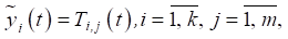 (5)
(5)
where k — number of temperature sensors; m — number of parameters of the thermal model.
Step response generation was performed in the ANSYS Mechanical module using the Application Customization Toolkit (ACT) extension, which supported the implementation of user scenarios. This made it possible to develop a software script in the Python programming language to automatically generate a special set of files containing independent step responses [14].
The analytical solution was performed on the basis of the state-space method through constructing a model of thermal characteristics according to the formula:
 (6)
(6)
where  — derivative of state vector over time t; y and u — vectors of output and input data, respectively; A, B, C, D — matrices of constant coefficients.
In equation (6), vector x = (x1, x2, …, xN)T contains state variables, input vector u = (qv1, qv2, Q1, Q2, qn1, qn2, T01, T02, …, T0k)T — values of the parameters of the thermal model (boundary and initial conditions), output vector y = (T1, T2, …, Tk)T — values of thermal characteristics.
The transfer function model is expressed by the following equation:
 (7)
(7)
where H — matrix complex transfer function.
Matrix transfer function H is obtained through applying the Laplace transform to formula (6), which is expressed by the following equation:
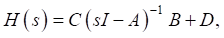 (8)
(8)
where s — Laplace complex variable; I — unity diagonal matrix.
Transfer function (8) reflects the dependence of the Laplace transform of output variable Y(s) = H(s)U(s) on the Laplace transform of the input variable U(s) of model (6) under zero initial conditions x(0) = x0 = 0. In this case, the dimension of the transfer function matrix H depends on the output value k = 4 and the dimension of the input value m = 10, which corresponds to the dimension of the initial step response (5). Therefore, model (6) is brought into line with the behavior of the source thermal model through approximating its transfer function (7) to step response (5) using the vector approximation method [15].
To construct the coefficient matrices of model (6), a reverse transition is performed from transfer function (8) to the model in the state space. In this case, transfer function (8) takes the form of the equation, whose denominator contains a characteristic polynomial of degree l = 4 (the order of the system), and the numerator contains a polynomial of degree z = l – 1:
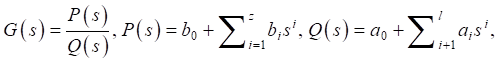 (9)
(9)
where a and b— coefficients of polynomials Q(s) and P(s), respectively.
The roots of polynomials Q(s) and P(s) represent the poles and zeros of transfer function (8), respectively. The method of indefinite multipliers is applied to equation (9) to decompose each element of matrix H into elementary fractions. Denoting the poles of the characteristic polynomial by  , we obtain an equation of the following form:
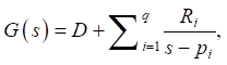 (10)
(10)
where
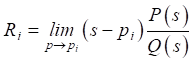 — matrix of dimension (k × m); q — number of poles.
The rank of matrix Ri is denoted by ri, and its decomposition into the product of two matrices with the full rank of the column and row, respectively, is performed:
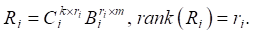 (11)
(11)
The matrices of model (6) are diagonal, of dimension An×n, Bn×m, Ck×n, Dk×m (n = 56) and contain elements that are obtained directly from the coefficients of transfer function (10).
System matrix A and control matrix B contain the following coefficients:
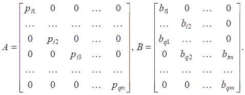 (12)
(12)
Output matrix C and feed forward matrix D contain the following coefficients:
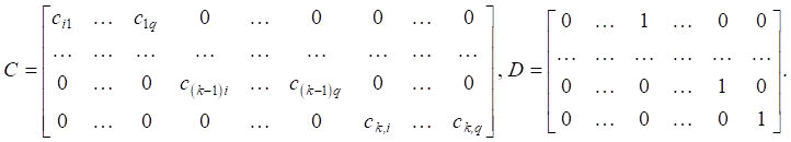 (13)
(13)
This approach makes it possible to perform the transition from a model in the form of transfer function (8) to a model in state space (6). The transition algorithms are also implemented in the MATLAB engineering calculation system of The MathWorks, Inc. (USA), in the form of special functions «ss2tf()» and «tf2ss()».
To obtain the values of thermal characteristics, the Cauchy problem is solved for a system of ordinary differential equations, since in formula (6), variable  is a derivative of the vector of states of the temperature field in time t. The solution to system of equations (6) is obtained using the fourth-order Runge-Kutta method.
Verification of the constructed analytical model was performed through conducting a series of computational experiments using an application program developed in the MATLAB system, which included the implementation of the fourth-order Runge-Kutta method (Fig. 3). Computational experiments were conducted on a personal computer (AMD Ryzen 5 5600U processor with Radeon Graphics 2.30 GHz, RAM 16.0 GB, system type 64-bit Windows 10 Pro version 21H2 operating system), whose characteristics were basic for modern computing technology.
The constructed analytical model and the application of the fourth-order Runge-Kutta method for solving a system of differential equations made it possible to calculate the values of thermal characteristics with high accuracy (Fig. 3). Due to the fact that the maximum error values, i.e., the difference between the model values of thermal characteristics obtained using numerical (FE-Model) and analytical (LTI-Model) solutions, did not exceed 0.72 °C over the entire modeling interval.
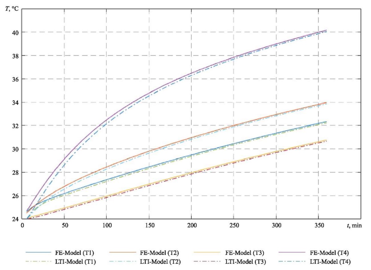
Fig. 3. Graphs of thermal characteristics in MATLAB system
Linear and Time-Invariant (LTI) Reduced Order Model (ROM) was developed in the ANSYS Twin Builder module of the ANSYS engineering analysis system based on the object's temperature field and the step response generated in the ANSYS Mechanical module.
The implementation of the digital model of thermal characteristics based on a temperature field using vector approximation consists in the sequential execution of seven main stages.
Stage 1. Importing a geometric model of an object and building a thermal model in an engineering analysis system.
Stage 2. Calculation of the object's temperature field based on the developed thermal model.
Stage 3. Generation of an independent step response based on the results of numerical modeling of the thermal characteristics of the object.
Step 4. Application of the vector approximation algorithm to obtain the poles and zeros of the transfer function of the state space model.
Stage 5. Building a model of the state space based on a known transfer function.
Stage 6. Development of a computer model of thermal characteristics.
Stage 7. Implementation of the digital model of the object.
Thus, the proposed digital model containing a computer model for an accurate assessment of the thermal characteristics of complex technical design objects was obtained through sequential completing all the above steps.
Research Results. The developed computer model (Thermal_SG400V_SML1) contains 6 inputs and 4 outputs (Fig. 4); this provides identifying the relationship between the parameters of the thermal model and the values of thermal characteristics. The volume heat release power (qv1, qv2), heat flows (Q1, Q2) and heat flux densities (qn1, qn2) were taken as input data of the computer model. The output data were thermal characteristics (T1–T4). The computer model is part of the digital model (Fig. 4 a) of thermal characteristics implemented in the ANSYS Twin Builder module.
The values of the parameters of the digital model, presented in the tabular form (Fig. 4 c), are fed to the input of the computer model (Fig. 4 a) using the STEP components. The graphic module shows the values of thermal characteristics (Fig. 4 b) obtained at the output of the computer model.
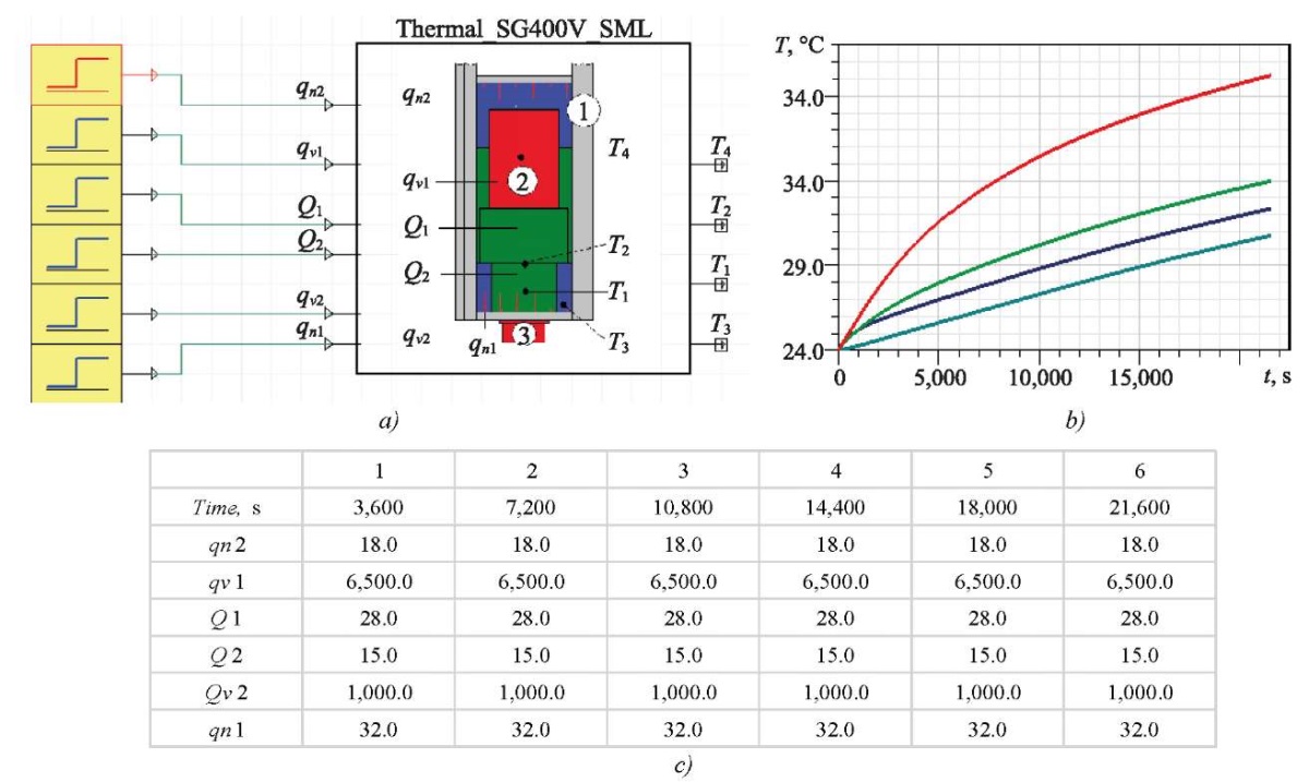
Fig. 4. Implementation of digital model in Ansys Twin Builder system:
a — computer model of thermal characteristics;
b — module for graphical representation of results;
c — module for monitoring input data of the computer model
During the development of the computer model, the limits of dimension from 2 to 4 orders, values of the target error ε = 5×10⁻³, and the tolerance for the zero order ε0 = 2×10⁻³ were set. The remaining parameters were set automatically, since the vector approximation method was as automated as possible in comparison to other methods that were supported in the ANSYS Twin Builder module.
In the process of developing a computer model, the ANSYS Twin Builder module automatically generated a special matrix of approximation errors 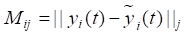 in the time domain, each element of which reflected the difference between the values of the thermal characteristics of step response (5) and transfer function (7) of the model in the state space. It is expressed by the following equation:
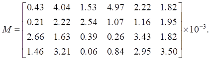 (14)
(14)
In this case, the maximum relative error did not exceed value ε = 4.97 × 10⁻³. At the same time, all other error values turned out to be less than the specified limit ε = 5 × 10⁻³. Zero-error value in matrix (14) meant that the input was ignored due to a very small contribution.
The estimation of the accuracy of the calculation of thermal characteristics using the proposed digital model was carried out through comparative analysis of the results obtained using numerical and analytical solutions. The comparative analysis was performed according to the criterion of maximum error. Maximum error ΔTmax, i.e., the difference between the values of thermal characteristics obtained using numerical and analytical solutions for all temperature sensors, was calculated at each time by the formula:
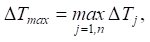 (15)
(15)
where ΔTj = |Tj,f – Tj,d| — error; Tj,f and Tj,d — temperature values of the finite element and digital models, respectively  m — number of temperature sensors.
To assess the digital model accuracy, an error calculation was performed, whose results were presented in the form of a surface (Fig. 5 a) and a linear graph (Fig. 5 b) of the maximum time error. The surface (Fig. 5 a) represented the calculated error values for each temperature sensor (dT1, dT2, dT3, dT4) individually and at each time point over the entire simulation interval.
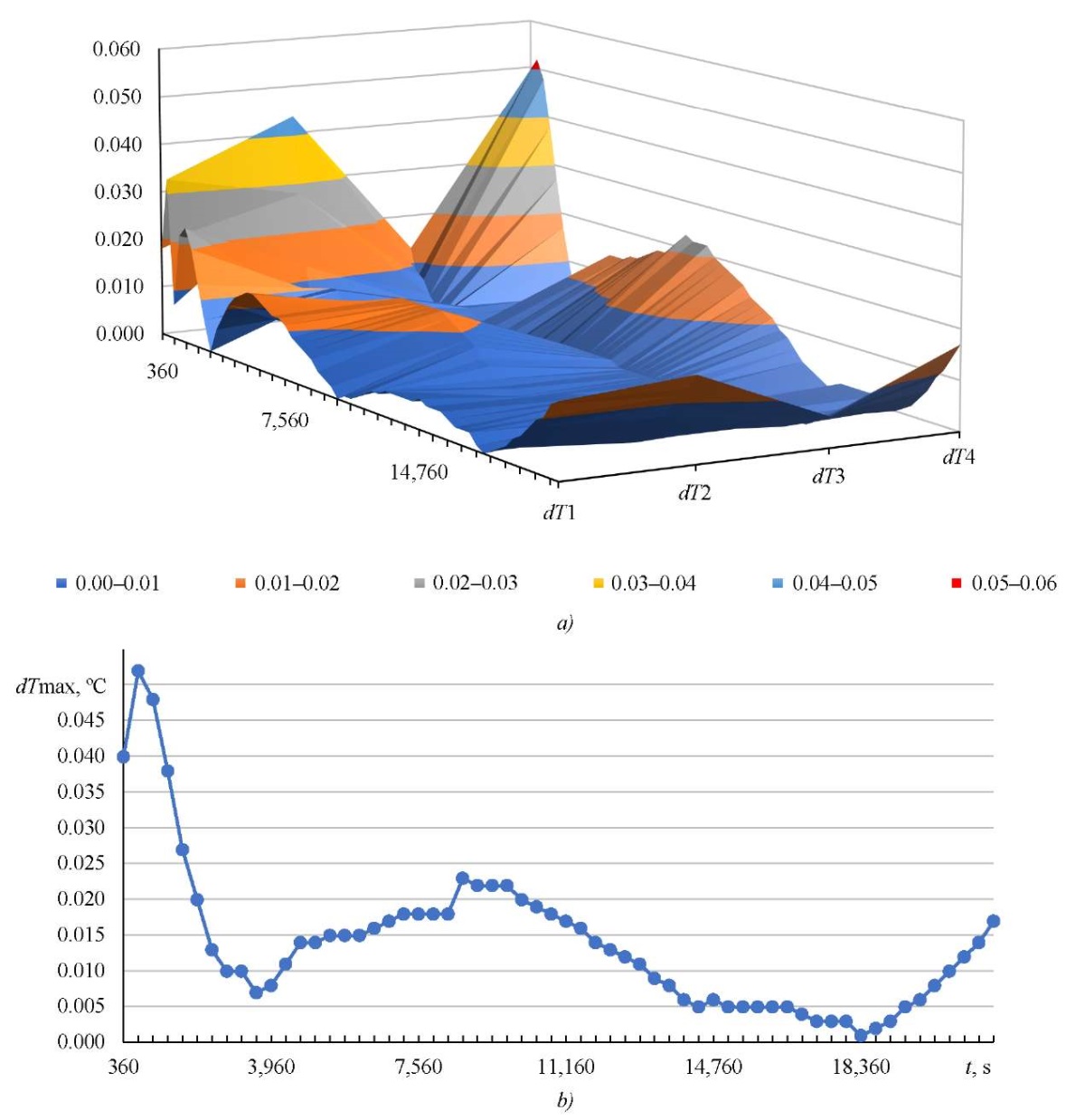
Fig. 5. Errors in the calculation of thermal characteristics:
a — error for each temperature sensor;
b — maximum error for all temperature sensors
The graph (Fig. 5 b) showed that for the selected time interval, maximum errorΔTmax did not exceed 0.1 °C. The error in calculating the thermal characteristics for each temperature sensor separately (Fig. 5 a) did not exceed the specified limits either.
Discussion and Conclusion. The obtained results of computational experiments and the conducted comparative analysis confirm the efficiency of the proposed digital model, which provides calculating thermal characteristics with high accuracy ΔTmax = 0.052 °С, for further analysis and identification of the thermal model.
The temperature field of the design object is influenced by many factors, which complicates the determination of the nominal values of thermal boundary conditions. To solve this problem, the study first analyzes the key technologies involved in the implementation of the digital twin of a complex technical object, then builds a thermal model and a computer reduced-order model LTI ROM of the transient temperature field. The developed computer model is used as part of a digital model that provides obtaining an accurate assessment of the thermal characteristics of the design object and thereby increases the efficiency of design procedures in the process of computer-aided design of complex technical facilities.
The accuracy and efficiency of calculations of the reduced-order computer model and the source full-order thermal model are evaluated by comparative analysis of the simulation results. The results of computational experiments show that, from the point of view of calculation accuracy, computer models of reduced order and finite element models of full order are generally comparable in accuracy, the maximum calculation error is within the acceptable range and does not exceed 0.1°C.
The results obtained during computational experiments do not contradict the results presented in the sources of scientific literature on similar topics and allow us to conclude that the use of the proposed digital model is effective for evaluating the thermal characteristics of complex technical objects in real time, which is one of the most important conditions for the implementation of digital twin technology.
However, changes in the temperature field of a complex technical facility still depend on many factors. Therefore, in further research, it is necessary to develop computer models of thermal deformations and conduct effective optimization algorithms based on artificial intelligence to provide the reliability of simulation results obtained using digital twins.
1. Bushuev VV, Kuznetsov AP, Sabirov FS, Khomyakov VS, Molodtsov VV. Precision and Efficiency of Metal-Cutting Machines. Russian Engineering Research. 2016;36:762–773. https://doi.org/10.3103/S1068798X16090070
2. Jianying Xiao, Kaiguo Fan. Research on the Digital Twin for Thermal Characteristics of Motorized Spindle. The International Journal of Advanced Manufacturing Technology. 2022;119:5107–5118. https://doi.org/10.1007/s00170-021-08508-y
3. Haoran Yi, Kaiguo Fan. Co-Simulation-Based Digital Twin for Thermal Characteristics of Motorized Spindle. The International Journal of Advanced Manufacturing Technology. 2023;125(9–10):4725–4737. https://doi.org/10.1007/s00170-023-11060-6
4. Kuo Liu, Lei Song, Wei Han, Yiming Cui, Yongqing Wang. Time-Varying Error Prediction and Compensation for Movement Axis of CNC Machine Tool Based on Digital Twin. IEEE Transactions on Industrial Informatics. 2022;18(1):109–118. https://doi.org/10.1109/TII.2021.3073649
5. Kurganova N, Filin M, Cherniaev D, Shaklein A, Namiot D. Digital Twins’ Introduction as One of the Major Directions of Industrial Digitalization. International Journal of Open Information Technologies. 2019;7(5):105–115. http://injoit.org/index.php/j1/article/view/748
6. Jones D, Snider C, Nassehi A, Yon J, Hicks B. Characterising the Digital Twin: A Systematic Literature Review. CIRP Journal of Manufacturing Science and Technology. 2020;29A:36–52. https://doi.org/10.1016/j.cirpj.2020.02.002
7. Aumann Q, Benner P, Saak J, Vettermann J. Model Order Reduction Strategies for the Computation of Compact Machine Tool Models. In: Proc. 3rd International Conference on Thermal Issues in Machine Tools. Cham: Springer; 2023. P. 132–145. https://doi.org/10.1007/978-3-031-34486-2_10
8. Mirzaev DA, Okishev KYu, Mirzoev AA. A Simple Analytical Model of Thermal Fields to Develop Digital Twins in Industrial Arc Welding. Vestnik of South Ural State University. Series: Mathematics. Mechanics. Physics. 2023;15(1):76–86. https://doi.org/10.14529/mmph230109
9. Bordatchev EV, Lapshin VP. Mathematical Temperature Simulation in Tool-to-Work Contact Zone during Metal Turning. Advanced Engineering Research (Rostov-on-Don). 2019;19(2):130–137. https://doi.org/10.23947/1992-5980-2019-19-2-130-137
10. Schröder C, Matthias V. Balanced Truncation Model Reduction with a Priori Error Bounds for LTI Systems with Nonzero Initial Value. Journal of Computational and Applied Mathematics. 2023;420:114708. https://doi.org/10.1016/j.cam.2022.114708
11. Xaver Thiem, Kauschinger B, Ihlenfeldt S. Online Correction of Thermal Errors Based on a Structure Model. International Journal of Mechatronics and Manufacturing Systems. 2019;12(1):49–62. https://doi.org/10.1504/IJMMS.2019.097852
12. Klochkov YuV, Nikolaev AP, Ishchanov TR, Andreev AS. FEM Vector Approximation for a Shell of Revolution with Account for Shear Deformations. Journal of Machinery Manufacture and Reliability. 2020;49:301–307. https://doi.org/10.3103/S105261882004007X
13. Xiao Hu, Scott Stanton, Long Cai, Ralph E White. A Linear Time-Invariant Model for Solid-Phase Diffusion in Physics-Based Lithium Ion Cell Models. Journal of Power Sources. 2012;214:40–50. https://doi.org/10.1016/j.jpowsour.2012.04.040
14. Polyakov AN, Pozevalkin VV. Software Module for Generating Input Data for Building Digital Models. RF Certificate of State Registration of a Computer Program, no. 2023660032. 2023. 1 p. (In Russ.).
15. Gourary MM, Zharov MM, Rusakov SG, Ulyanov SL, Khodosh LS. An Effective Algorithm for Realization of the Vector Fitting Method for the Identification Tasks of the Dynamical Systems. Mechatronics, Automation, Control. 2015;16(9):579–584. https://doi.org/10.17587/mau.16.579-584
Vladimir V. Pozevalkin, Cand.Sci. (Eng.), Senior Lecturer of the Applied Computer Science in Economics and Management Department
13, Pobedy Ave., Orenburg, 460018
Alexander N. Polyakov, Dr.Sci. (Eng.), Professor, Head of the Department of Technology of Mechanical Engineering, Metalworking Machines and Complexes
13, Pobedy Ave., Orenburg, 460018
Pozevalkin V.V., Polyakov A.N. Implementation of a Digital Model of Thermal Characteristics Based on the Temperature Field. Advanced Engineering Research (Rostov-on-Don). 2024;24(2):178-189. https://doi.org/10.23947/2687-1653-2024-24-2-178-189. EDN: EYQXQZ


Advanced Engineering Research (Rostov-on-Don)
ISSN 2687-1653 (Online)
Contact with: Publisher / Editorial Office of the Journal
Publisher: Don State Technical University - DSTU, Rostov-on-Don, Russia - https://donstu.ru/en/
Editor-in-Chief: Alexey N. Beskopylny, Dr.Sci. (Eng.), Professor, Vice-Rector, Don State Technical University (Rostov-on-Don, Russia)
Don State Technical University
1, Gagarin Sq., Rostov-on-Don, 344003, Russia
tel.: +7 (863) 2738-372, e-mail: vestnik@donstu.ru
16+
Processing of personal data