Contents
Scroll to:
https://doi.org/10.23947/2687-1653-2025-25-3-186-196
EDN: HCPJJV
Scroll to:
Introduction. Modern development of exoskeletons opens new horizons for rehabilitation and improving the quality of life of people with limited mobility. The relevance of the study on methods of optimal control of exoskeletons is due to the growing demand in medicine and industry. However, there are numerous challenges related to the efficient control of exoskeletons, especially in the context of the integration of elastic elements. Topics related to optimal control and tuning of system parameters to reach maximum efficiency and user comfort remain insufficiently studied. The objective of this study is to develop a method of optimal control of a lower limb exoskeleton (LLE) with elastic elements while optimizing energy costs and accounting for external disturbances.
Materials and Methods. The LLE is represented by a simplified model of an inverted pendulum with elastic elements in the feet. The dynamic model of the LLE was developed using Lagrange equations. The optimal control method was based on the synthesis of a linear quadratic regulator designed to minimize energy costs. To account for the influence of external disturbances, a Kalman filter was integrated into the control loop. The parameters of the mathematical model of the LLE were obtained from published data. System simulation was performed in the Wolfram Mathematica environment.
Results. A method of optimal control of the LLE with elastic elements has been developed. This method optimizes energy costs while maintaining vertical equilibrium. The system was modeled using optimal terminal control, followed by optimal feedback control. During feedback control, key parameters affecting system stability were identified: spring stiffness and damping coefficients. Integration of the Kalman filter enabled compensation for external disturbances.
Discussion. The use of terminal control within the developed method reduced energy costs by 98% within a specified stabilization timeframe. Optimal values of spring stiffness and damping coefficients for obtaining the best system response were identified. The use of the optimal control method of the LLE in combination with the Kalman filter confirmed the effective compensation of external disturbances and noise, which provided the convergence of transient processes with minimal energy consumption.
Conclusion. The proposed method for achieving optimal control while minimizing energy costs is a promising solution in the field of control signal calculation required to ensure stability and determine the optimal energy cost function. This is especially true for medical rehabilitation tasks. These results may be useful for further research and development in the field of robotics and wearable devices.
Deeb D., Merkuryev I.V. Optimal Control Method for a Lower Limb Exoskeleton with Elastic Elements. Advanced Engineering Research (Rostov-on-Don). 2025;25(3):186-196. https://doi.org/10.23947/2687-1653-2025-25-3-186-196. EDN: HCPJJV
Introduction. Lower limb exoskeletons (LLE) are of increasing interest due to the need to address global health issues, such as aging population and increase in neuromuscular injuries [1]. These devices are designed to provide effective solutions to support and improve human motor functions, such as walking assistance [2], rehabilitation and compensation for loss of balance [3], thereby increasing independence and quality of life.
LLE are often designed without elastic elements due to the increased complexity of the stabilization during movement and the influence of additional factors that arise when using elastic elements [4]. On the other hand, these exoskeletons may require elastic elements that improve the ability of the structure to adapt to uneven surfaces. Elastic elements can be installed in the ankle area [5] or used to completely replace it [6].
LLE control is a complex task. Various approaches to its solution have been proposed previously. The development of an effective control method depends on numerous factors, maintaining the constant relevance of research in this area. There are different methods for LLE control: adaptive control method [1][7], robust (stable) methods [8][9], and optimal control method [10][11]. Despite the efficiency of the first two methods, the third is the most successful. The optimal control method takes into account not only the increase in the stability and efficiency of LLE control under dynamic and unpredictable conditions, but also allows for reducing energy costs and the consumption of resources of the control system [10][11]. However, the integration of elastic elements into the LLE feet causes complications in their control. In addition, taking into account external disturbances when controlling the LLE is accompanied by new problems in providing the dynamic stability of the LLE control system.
Based on the above, it can be argued that there is a need to develop a method for optimal control of LLE with elastic elements. Therefore, the objective of this study was to develop a method for optimal control of the lower limb exoskeleton and elastic elements while optimizing energy costs and taking into account external disturbances. This method allows minimizing the quadratic function of energy costs in the presence of elastic elements and external disturbances.
One of the factors that further complicates the solution to the issue of dynamic stability of LLE is the presence of white noise, which is an interference to the control signal [12], which is investigated in this work.
To achieve the stated goal, the following tasks were set:
Materials. To develop a mathematical model of the LLE with elastic elements in the feet, its kinematic scheme is considered. The foot is represented by elastic elements and is connected to the model by the type of an inverted pendulum (Fig. 1). The model includes inertial properties, kinematic limitations of the joints, and external forces acting on the system.
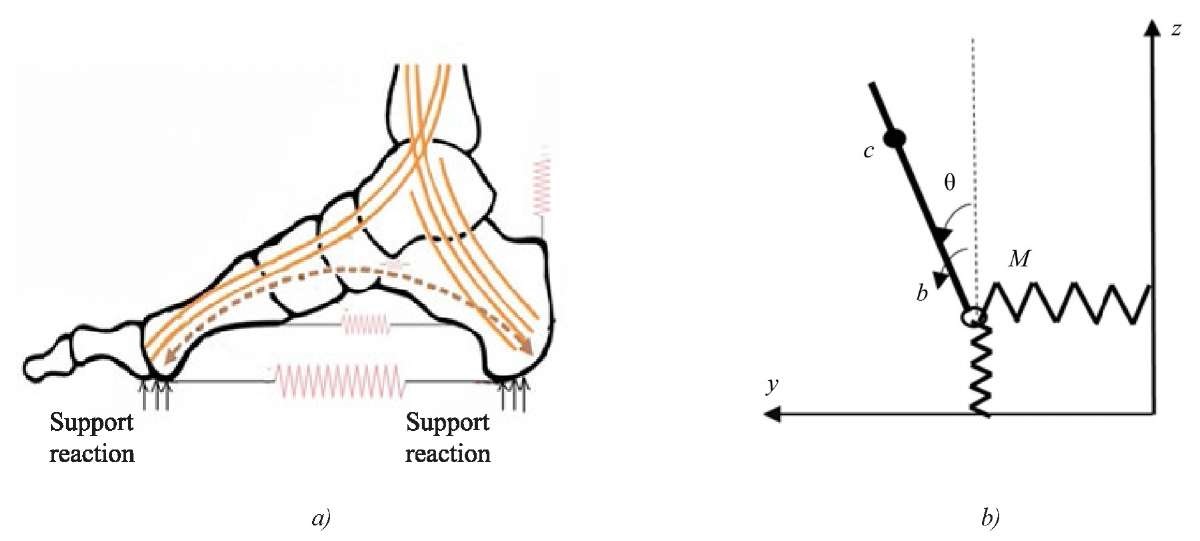
Fig. 1. Kinematic scheme of LLE:
a — biomechanical model of physiological “foot spring”1;
b — simplified dynamic model of exoskeleton:
c — center of mass; θ — angle of ankle joint; M — control moment
The characteristics of the elastic elements and the parameters of the model are as follows: ky, kz — stiffness coefficients of the horizontal and vertical springs, respectively. Their values — ky ∈ [ 500, 1500] N/m [13], kz ∈ [ 7000, 20000] N/m [14]. cy, cz — horizontal and vertical damping coefficients, respectively, cy ∈ [ 30, 200 N∙s/m], cz ∈ [ 500–2000 N∙s/m] [15].
 — moment of exoskeleton inertia relative to the center of mass, kgm²; m = 70 — mass of exoskeleton with patient, kg; h = 1 — length of exoskeleton to the center of mass, m; μy = 0.7 and μz = 0 — friction coefficients; Ny = 0 and Nz = m g — normal forces, N; g = 9.8 — acceleration of gravity, m/s².
Methods. The dynamics of the LLE is described by the Lagrange equations of the second kind in general form2:
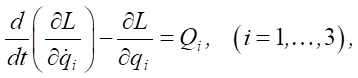 (1)
(1)
where L = T – V — Lagrange function; T — kinetic energy of the system; V — potential energy of the system; Q — generalized forces; q = (θ, yb, zb)T — vector of generalized coordinates;  — rotary angle of exoskeleton link, measured from horizontal surface (parallel to reference plane) in counterclockwise direction; yb, zb — horizontal and vertical displacement of the base.
The coordinates of the center of mass of the pendulum are determined by the following equations:
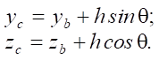 (2)
(2)
The kinetic energy of a pendulum is given by the formula:
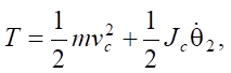 (3)
(3)
where v — speed of the center of mass, it is equal to  .
.
The potential energy of the systems is described by the following equation:
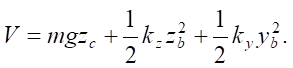 (4)
(4)
The generalized damping forces applied through the Rayleigh dissipation function to simulate linear damping are written as [15]:
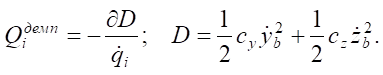 (5)
(5)
The Coulomb friction model is given by the following equations [15]:
 (6)
(6)
where α >> 1 — regularization parameter (for approximating the discontinuous function sign(v)), in this paper, α = 100 is selected.
After intermediate calculations, equations (2–6) take the form:
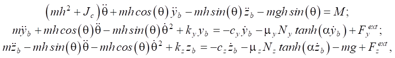 (7)
(7)
where  — external generalized forces.
In the vicinity of vertical equilibrium (θ ≈ 0), assumptions are valid: sin θ ≈ θ, cos θ = 1, zb ≈ –mg/kz. Equations (7) are linearized taking into account smallness  and
and  at low speeds:
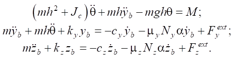 (8)
(8)
Under the assumptions of small angles, the vertical displacement of z becomes dynamically independent of horizontal y and angular θ states. Its behavior is reduced to a harmonic oscillator, which can be analyzed separately [12].
For control synthesis, we present the system in the canonical form of the state space, taking into account external disturbances and measurement noise. Given the state vector  , we write the system in the Cauchy form:
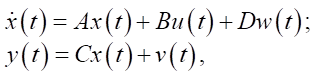 (9)
(9)
where A — state matrix; B — control matrix; u(t) — vector of control signals; D — matrix of disturbances; w(t) — vector of external disturbances; C — matrix of measurements; v(t) — vector of external disturbances.
The main task of the regulator is to transfer the dynamic system from the initial state x(t0) to the specified final state x(t1) in a certain time t1.
Controllability Gramian W characterizes the ability of the system to reach arbitrary states in a finite time T and is determined by the formula [12]:
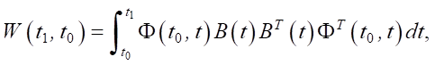 (10)
(10)
where Ф(t0, t) = eA(t0 – t) — matrix exponent.
The system is fully controllable on [t0, t1] if and only if W(t1, t0) is invertible. If the Gramian is invertible, any state xT ∈ ℝn can be reached using the appropriate control u(t) [12].
The control that minimizes the quadratic function of energy consumption and transfers the system from state x(t0) to state x(t1), has the form [12]:
 (11)
(11)
After intermediate calculations, the quadratic function of energy consumption can be calculated using expression (12):
 (12)
(12)
The control given by equation (11) is programmatic (open-loop) and time-dependent. To provide asymptotic stabilization of the system at the origin of coordinates under arbitrary initial conditions, it is required to synthesize the closed-loop control law based on real-time feedback. The control task is formulated in the form of minimizing the quadratic function of energy consumption [12]:
 (13)
(13)
where R — positive definite matrix; Q — positive semi-definite matrix.
Optimal control that minimizes energy costs can be implemented as a negative feedback with variable parameters:
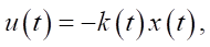 (14)
(14)
where k(t) = R–1BTP(t); k(t) — feedback coefficient matrix; P(t) — solution to the Riccati equation.
To find P(t) as t → ∞, it is required to solve the algebraic Riccati equation, which is given as follows:
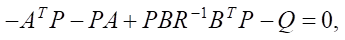 (15)
(15)
The system with control signal u(t) is described by the equation:
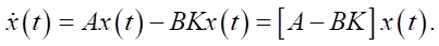 (16)
(16)
In practice, measuring all states is impossible due to the limited number of sensors, noise and measurement errors [12]. To estimate the state vector from the inputs and outputs, an optimal Kalman filter is used.
The system with control signal u(t) and Kalman filter for determining the state vector has the following form [12]:
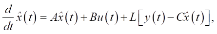 (17)
(17)
where  — estimated state;
  — observer output; L — Kalman gain matrix.
In the presence of external disturbances w(t) and measurement noise v(t) with zero mathematical expectations M[v(t)] = 0, M[w(t)] = 0 and covariance matrices sw and sv, respectively, gain matrix L is determined from the solution to the algebraic Riccati equation (18), and, accordingly, stationary Kalman filter is found:
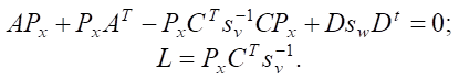 (18)
(18)
Control of a linear non-stationary system with external disturbances at the input and output is implemented using linear feedback on the state estimate:
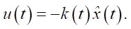 (19)
(19)
The type of closed-loop system with feedback for estimating the state vector is determined by the formula:
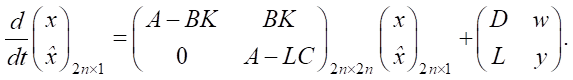 (20)
(20)
After developing the optimal control method for LLE with elastic elements and taking into account the impact of external disturbances, it remains to perform numerical modeling and analysis of the obtained results of the study on transient processes for the angle of deviation and displacement. For this purpose, at the first stage, the optimal control method is focused on restoring equilibrium for a certain stabilization time without taking into account the intermediate trajectory of motion. At the second stage, the optimal feedback control method is used to find the optimal intermediate trajectory of motion both with and without the Kalman filter.
Research Results. The paper investigates the transient processes of the control moment, force, displacement and angle during the transition of the LLE with elastic elements from an unstable position to a vertical equilibrium position. The results of numerical modeling are shown in Figures 2–6 for three initial conditions: Y1 = [ 1/10, 0, 0 ,0], Y2 = [ 1/10, 0, 1/10 ,0], Y3 = [ 1/10 0 1/10 0 0 1/10 0 1/20 0].
The results of terminal control are calculated for a stabilization time of 0.6 s. Figure 2 shows the curves of the control moments of the open-loop system under the initial conditions Y1 and the target position in the vertical equilibrium state. The blue curve corresponds to control moment M, the orange one — to control force Fy.

Fig. 2. Open-loop control signal curves
The values of the quadratic function of energy consumption for terminal control for different values of stabilization time are calculated using equation (12) and are presented in Table 1. A decrease in the value of the function of energy consumption with an increase in stabilization time can be noticed.
Table 1
Values of Quadratic Energy Consumption Function
|
Stabilization time, s |
0.1 |
0.2 |
0.3 |
0.4 |
|
Value of quadratic function of energy consumption (J) |
1,648.8 |
212.1 |
66.1 |
29.9 |
Figure 3 shows the curves of transient processes of the key parameters of the dynamic LLE system (θ, yb) under the initial conditions Y1. The blue curve represents the transient process of the deviation angle θ, and the orange curve — change in the coordinate along the ordinate axis yb during the specified stabilization time of 0.6 s under terminal control.

Fig. 3. Transient response curves
The simulation results in Figures 4–6 are obtained using the feedback control type, which allows searching for the optimal intermediate trajectory of motion. To study the impact of the elastic elements’ stiffness (changes in spring stiffness coefficient ky) on the stability of the dynamic LLE system while minimizing energy costs, transient processes of the key parameters of the dynamic LLE system (Fig. 4) were considered under the initial conditions Y2 and the following parameters of the feedback system: cy = 100, kz = 20,000, Q = eye(4) ⋅ 10³, R = eye(2).
The orange line represents  dependence, and the green line —
  . The following values of the stiffness coefficient are selected: ky = [ 700, 1000, 1500] N/m. The transient processes are shown in Figure 4 a, b, c, respectively.
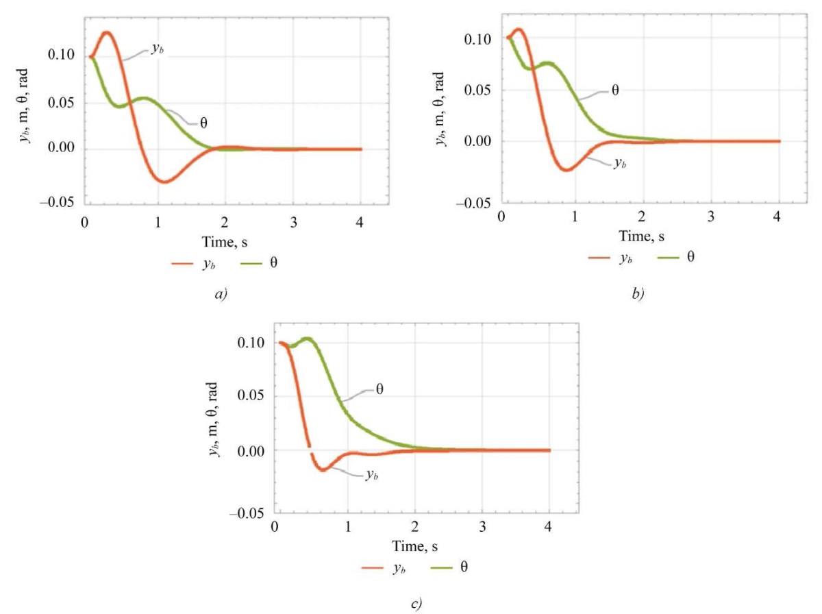
Fig. 4. Transients when changing the spring stiffness coefficient:
a — at ky = 700 and cy = 100;
b — at ky = 1000 and cy = 100;
c — at ky = 1500 and cy = 100
To study the effect of damping of elastic elements (changes in damping coefficient cy) on the stability of the dynamic LLE system while minimizing energy costs, transient processes of the key parameters of the dynamic LLE system(θ, yb) (Fig. 5) are considered under the initial conditions Y2 and ky =1000 with feedback. The orange line represents the yb dependence, and the green line — θ. The damping coefficient values are cy = [ 0, 50, 100] N∙s/m, and the transient processes are shown in Figure 5 a, b and c, respectively.
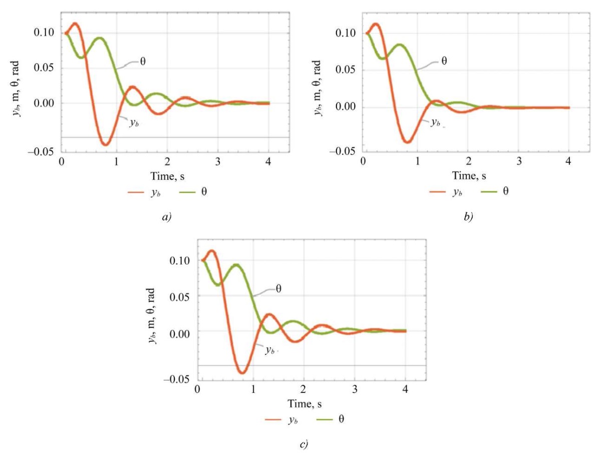
Fig. 5. Transients of damping coefficient variation:
a — at cy = 0 and ky =1000;
b — at cy = 0 and ky =1000;
c — at cy = 100 and ky =1,000
This research also takes into account the effect of noise through adding Kalman filter. Figure 6 shows the transient response curves under the initial conditions Y3 = [ 1/10 0 1/10 0 0 1/10 0 1/20 0] and the covariance matrices sw = eye(1) and sv = 0.1 eye(2). The orange line illustrates the transient response yb, and the green line — transient response θ.
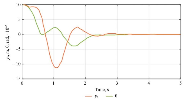
Fig. 6. Transient response curves using Kalman filter
Discussion. To achieve the research objective, the previous section presented the simulation results obtained using the proposed optimal control method to minimize energy costs during the transition of the studied LLE from an unstable position to a vertical equilibrium position.
Table 1 shows that as the time required to reach the target stable state increases, energy costs decrease proportionally. This dependence is consistent with the dynamics of control signals: as the permissible stabilization time increases, the amplitudes of the control moments M and  decrease, which, according to formulas (12)–(14), reduces the energy costs. It can be concluded that an increase in the stabilization time (within 0.1–0.4 seconds) reduces energy costs by 98%.
The curves in Figure 3 demonstrate a transient process lasting 0.6 s before reaching the vertical equilibrium position, which is consistent with the principles of terminal control (reaching the target stable state within a certain stabilization time).
The curves in Figure 4 illustrate the effect of changing the stiffness coefficient on the transient processes of the key parameters of the LLE dynamic system (θ, yb). Changing the coordinate along the ordinate axis yb at a low value of the stiffness coefficient is characterized by significant overshoot and slow stabilization, and an increase in the stiffness coefficient eliminates overshoot and accelerates the stabilization of the system. On the contrary, changes in angle θ demonstrate an inverse relationship: at a low value of the stiffness coefficient, a smooth transient process without overshoot and a short stabilization time of the system are observed, while an increase in the stiffness coefficient to 1500 causes overshoot in the angle, despite accelerated stabilization. This contradiction emphasizes the competing dynamics between yb and θ. At the stiffness coefficient ky =1000 (Fig. 4 b), an optimal compromise is reached: minimization of overshoot in the coordinate yb, maintaining the stability of angle θ and fast convergence. This mode provides balanced operation of the system.
The reliability of the results obtained is validated by the stability of the closed system, which is confirmed by the negative real parts of its poles for all the studied values of the stiffness coefficient given in Table 2.
Table 2
Poles of a Closed System
|
Process option |
K y |
Poles of closed system |
|
1 |
700 |
–2.2445 + 3.8530i –2.2445 – 3.8530i –4.5071 – 3.2807i |
|
2 |
1000 |
–2.6133 + 5.4608i –2.6133 – 5.4608i –3.6385 – 3.1496i |
|
3 |
1500 |
–2.7679 + 7.5731i –2.7679 – 7.5731i –3.2042 – 3.0242i |
The curves in Figure 5 show the effect of the damping coefficient. At a low value of the damping coefficient, significant vibration of the system is observed before reaching the steady state, accompanied by overshoot. Increasing cy reduces the amplitude of vibrations and eliminates overshoot, but results in a growth of energy costs. To provide a balance between stability and the value of the quadratic function of energy costs, the value of coefficient cy = 100 is selected, which guarantees the stability of the LLE control system with elastic elements.
From the image in Figure 6, it follows that the Kalman filter provides the convergence of transient processes to zero values within three seconds when exposed to white noise, confirming its robust stabilizing properties.
The results obtained show the following picture. Firstly, the use of open control as a basic stage allows minimizing energy costs at the stage of bringing the system from an unstable state to the target vertical equilibrium at a given stabilization time. Secondly, the transition to closed loop control based on the state feedback provides asymptotic stability and stability of transient modes through solving the Riccati equation and implementing an effective Kalman filter. Thirdly, numerical modeling revealed an important effect of the parameters of elastic elements on the dynamics of the system: increasing the spring stiffness reduces overshoot in angle θ and accelerates stabilization, but it can cause difficulties on the way to a stable trajectory; increasing damping reduces vibrations and reduces overshoot, but increases energy costs. A balance between stability and energy costs is found, which is reached at specific values ky and cy (in the examples: ky = 1000 N/m, cy = 100 N·s/m).
Based on the previous discussion and analysis of the results obtained in the paper, it can be said that the developed method of optimal control of the LLE with elastic elements has managed to provide the stability of the control system of this exoskeleton for a certain stabilization time and with minimal energy consumption.
Conclusion. A technique for optimal control of a lower limb exoskeleton (LLE) with elastic elements in the feet, taking into account external disturbances and measurement noise, has been formulated and implemented. The main approach is based on representing the LLE dynamics as a system of Lagrange equations, translating it into a canonical form of the state space, and synthesizing the control law through optimization of quadratic functions of energy consumption and system stability. A Kalman filter was used to assess the state, which allowed for correct operation under conditions of a limited number of sensors and the presence of external disturbances.
The practical significance of the results consists in the development of a technique that allows adaptively selecting the parameters of elastic elements and the control mode depending on the conditions of the task and objectives (minimization of energy costs, acceleration of stabilization, minimization of overshoot). In terms of potential applications, this can help improve the efficiency of rehabilitation technologies, reduce energy consumption in prosthetic and orthotic systems, and improve the stability of movements on uneven surfaces. The prospects for the research include experimental verification of the technique and its adaptation to variable loads and complex surfaces, which is a challenge for medical rehabilitation and robotics.
1. Subbotin F. Biomechanics of the Foot. Part 1. Fidel Subbotin School; 2024. (In Russ.) URL: https://fs-school.ru/blog/988624 (accessed: 10.05.2025).
2. Lynch KM, Park FC. Modern Robotics: Mechanics, Planning, and Control: Video Supplements and Software. Cambridge University Press; 2017. URL: http://hades.mech.northwestern.edu/index.php/Modern_Robotics (accessed: 10.05.2025).
1. Yatsun SF, Loktionova OG, Khalil Hamed Mohammed Hamood Al Manji, Yatsun AS, Karlov AE. Simulation of Controlled Motion of a Person When Walking in an Exoskeleton. Proceedings of Southwest State University. 2019;23(6):133–147. https://doi.org/10.21869/2223-1560-2019-23-6-133-147
2. Habib Mohamad, Sadjaad Ozgoli. Online Gait Generator for Lower Limb Exoskeleton Robots: Suitable for Level Ground, Slopes, Stairs, and Obstacle Avoidance. Robotics and Autonomous Systems. 2023;160:104319. https://doi.org/10.1016/j.robot.2022.104319
3. Bottin-Noonan J, Sreenivasa M. Model-Based Evaluation of Human and Lower-Limb Exoskeleton Interaction during Sit to Stand Motion. In: Proc. IEEE International Conference on Robotics and Automation (ICRA). New York City: IEEE; 2021. P. 2063–2069. https://doi.org/10.1109/ICRA48506.2021.9561727
4. Shchurova EN, Prudnikova OG, Kachesova AA, Saifutdinov MS, Tertyshnaya MS. Improvement of Functional State of Patients after Spinal Cord Injury During Epidural Electrical Stimulation: Prospective Study. Bulletin of Rehabilitation Medicine. 2023;22(6):28–41. https://doi.org/10.38025/2078-1962-2023-22-6-28-41
5. Nuckols RW, Sawicki GS. Impact of Elastic Ankle Exoskeleton Stiffness on Neuromechanics and Energetics of Human Walking across Multiple Speeds. Journal of NeuroEngineering and Rehabilitation. 2020;17(1):75. https://doi.org/10.1186/s12984-020-00703-4
6. Orekhov G, Lerner ZF. Design and Electromechanical Performance Evaluation of a Powered Parallel-Elastic Ankle Exoskeleton. IEEE Robotics and Automation Letters. 2022;7(3):8092–8099. https://doi.org/10.1109/LRA.2022.3185372
7. Hamed Jabbari Asl, Tatsuo Narikiyo, Michihiro Kawanishi. Neural Network-Based Bounded Control of Robotic Exoskeletons without Velocity Measurements. Control Engineering Practice. 2018;80:94–104. https://doi.org/10.1016/j.conengprac.2018.08.005
8. Jinghui Cao, Sheng Quan Xie, Raj Das. MIMO Sliding Mode Controller for Gait Exoskeleton Driven by Pneumatic Muscles. IEEE Transactions on Control Systems Technology. 2017;26(1):274–281. https://doi.org/10.1109/TCST.2017.2654424
9. Madani T, Daachi B, Djouani K. Non-Singular Terminal Sliding Mode Controller: Application to an Actuated Exoskeleton. Mechatronics. 2016;33:136–145. https://doi.org/10.1016/j.mechatronics.2015.10.012
10. Rigatos G, Abbaszadeh M, Pomares J, Wira P. A Nonlinear Optimal Control Approach for a Lower-Limb Robotic Exoskeleton. International Journal of Humanoid Robotics. 2020;17(5):2050018. https://doi.org/10.1142/S0219843620500188
11. Jun Chen, Yuan Fan, Mingwei Sheng, Mingjian Zhu. Optimized Control for Exoskeleton for Lower Limb Rehabilitation with Uncertainty. In: Proc. Chinese Control and Decision Conference (CCDC). New York City: IEEE; 2019. P. 5121–5125. https://doi.org/10.1109/CCDC.2019.8833418
12. Rigatos G, Busawon K. Robotic Manipulators and Vehicles: Control, Estimation and Filtering. Cham: Springer; 2018. 734 p. https://doi.org/10.1007/978-3-319-77851-8
13. Madhusudhan Venkadesan, Ali Yawar, Carolyn M Eng, Marcelo A Dias, Dhiraj K Singh, Steven M Tommasini, et al. Stiffness of the Human Foot and Evolution of the Transverse Arch. Nature. 2020;579:97–100. https://doi.org/10.1038/s41586-020-2053-y
14. Juanjuan Zhang, Collins SH. The Passive Series Stiffness that Optimizes Torque Tracking for a Lower-Limb Exoskeleton in Human Walking. Frontiers in Neurorobotics. 2017;11:68. https://doi.org/10.3389/fnbot.2017.00068
15. Tsapenko V, Tereshchenko M, Tymchik G, Matvienko S, Shevchenko V. Analysis of Dynamic Load on Human Foot. In: Proc. IEEE 40th International Conference on Electronics and Nanotechnology (ELNANO). New York City: IEEE; 2020. P. 400–404. https://doi.org/10.1109/ELNANO50318.2020.9088788.
Delshan Deeb, Postgraduate student, Teaching Assistant of the Department of Robotics, Mechatronics, Dynamics and Strength of Machines
14, Krasnokazarmennaya Str., Moscow, 111250
ScopusID 59000476600
Igor V. Merkuryev, Dr.Sci. (Eng.), Associate Professor, Head of the Department of Robotics, Mechatronics, Dynamics and Strength of Machines
14, Krasnokazarmennaya Str., Moscow, 111250
ScopusID 35422634900
A method for optimal control of a lower-limb exoskeleton with elastic elements in the feet is developed. It minimizes energy consumption while accounting for external disturbances and measurement noise. The method is based on the Lagrange model and control synthesis through solving the Riccati equation. It is shown that increasing the stabilization time significantly reduces energy consumption. An analysis of the effect of the stiffness and damping of the elastic elements has revealed a tradeoff between stabilization speed and overshoot. The use of a Kalman filter ensures robust state estimation and stable convergence in the presence of white noise.
Deeb D., Merkuryev I.V. Optimal Control Method for a Lower Limb Exoskeleton with Elastic Elements. Advanced Engineering Research (Rostov-on-Don). 2025;25(3):186-196. https://doi.org/10.23947/2687-1653-2025-25-3-186-196. EDN: HCPJJV


Advanced Engineering Research (Rostov-on-Don)
ISSN 2687-1653 (Online)
Contact with: Publisher / Editorial Office of the Journal
Publisher: Don State Technical University - DSTU, Rostov-on-Don, Russia - https://donstu.ru/en/
Editor-in-Chief: Alexey N. Beskopylny, Dr.Sci. (Eng.), Professor, Vice-Rector, Don State Technical University (Rostov-on-Don, Russia)
Don State Technical University
1, Gagarin Sq., Rostov-on-Don, 344003, Russia
tel.: +7 (863) 2738-372, e-mail: vestnik@donstu.ru
16+
Processing of personal data