Contents
Scroll to:
https://doi.org/10.23947/2687-1653-2025-25-4-2215
EDN: DWKVUM
Scroll to:
Introduction. With highway congestion increasing, the efficiency of intelligent transportation systems depends on highquality short-term traffic prediction. Statistical methods do not adequately account for nonlinear and dynamic traffic changes. Long short-term memory (LSTM) and support vector machines (SVR) offer more promising solutions. However, they are not ranked in terms of accuracy, as there are no studies comprehensively comparing their adequacy for shortterm traffic flow prediction. The proposed study fills this gap. The research objective is to compare the accuracy of LSTM and SVR, and select the optimal approach for traffic flow prediction on Shenzhen Meiguang Expressway.
Materials and Methods. Traffic detector data was collected on the Meiguan Expressway in June 2021. Data preprocessing methods were used, including weighted mean imputation and normalization. Autocorrelation analysis was used for feature extraction, along with the creation of an interaction variable between speed and detector occupancy. Models were trained and tested on data collected from detectors at 5-minute intervals.
Results. LSTM performed 17.86% better in terms of root mean square error, 19.82% better in terms of mean absolute error, and 25.78% better in terms of mean absolute percentage error. In periods with the lowest flow rate prediction error, RMSE, MAE, and MAPE for the LSTM model were 36.5%, 34.3%, and 42.3% lower, respectively. In periods with the highest error, RMSE, MAE, and MAPE for the LSTM model were 73.2%, 65.4%, and 64.4% lower, respectively. The Wilcoxon signed-rank test <0.05 confirmed the statistical significance of the differences.
Discussion. The superior predictive performance of LSTM stems from its architecture, namely, the combination of interaction variables and lag metrics. LSTM accounts better for flow time dependences, adapts to complex, long-term dynamic changes, and remains accurate even with significant fluctuations. The lower predictive performance of SVR stems from its weak, nonlinear approximation ability. Sudden flow changes increase significantly error rates.
Conclusion. When choosing between a neural network and a machine learning model for short-term traffic flow prediction on an expressway, the neural network model, such as LSTM, should be preferred. These research results can be useful in predictive strategies for reducing congestion. Short-term prediction based on LSTM can serve as a basis for optimizing traffic management, reducing congestion and pollutant emissions, and for optimizing intelligent transportation systems. A promising direction is the development of hybrid architectures that integrate contextual data (weather, infrastructure, accidents) to improve real-time predictions.
Topilin I.V., Han M., Feofilova A.A., Beskopylny N.A. Comparative Analysis of Neural Network and Machine Learning Models for Short-Term Traffic Flow Prediction on Shenzhen Expressway. Advanced Engineering Research (Rostov-on-Don). 2025;25(4):350-362. https://doi.org/10.23947/2687-1653-2025-25-4-2215. EDN: DWKVUM
Introduction. The solution to the pressing global problem of efficient traffic management relies on accurate traffic analysis and prediction. Urbanization and globalization are transforming and overburdening road transport systems, requiring fundamentally new and universal approaches to manage them. Obviously, neural network solutions and adequate machine models can provide such solutions. Their testing and training should be based on data obtained on high-speed highways in megacities. In this case, the results can be extrapolated to similar systems, i.e., major highways with heavy traffic.
This research utilized data collected in Shenzhen, a large city in southeastern China. With a population exceeding 17.5 million, motorization is growing at an annual rate of 8%. Consequently, the metropolis faces increasing congestion on its 386-kilometer-long highways1. The rapid development of the road network, on the one hand, contributes to significant economic growth in Chinese newest megacity, but on the other, it overloads the transport network and leads to disruptions [1]. Thus, Shenzhen problem is not a local anomaly, but a typical example of the “success disease” facing megacities worldwide. The current situation directly contradicts the following key UN Sustainable Development Goals (SDG)2.
SDG 3 “Good Health and Well-Being”. Congestion is not just a waste of time. It is a source of chronic stress, increased noise, and, most importantly, air pollution (PM2.5, NOx). According to the WHO, air pollution is one of the leading health risks.
It is important to note that the electrification of transport, which Shenzhen is actively promoting, is only part of the solution. Decarbonization by reducing the number of private cars is also needed.
SDG 9 “Industry, Innovation, and Infrastructure”. Chronic congestion reduces economic competitiveness of the city. Losses from congestion increase logistics costs, reduce labor productivity, and make areas less attractive for investment.
SDG 11 “Sustainable Cities and Communities”. Congestion makes cities unsustainable. It reduces the efficiency of urban systems, increases the time and cost of travel, impairs access to basic services (healthcare, education), and reduces quality of life.
SDG 13 “Climate Action”. The transport sector is a major source of greenhouse gases. Congestion significantly increases CO₂ emissions per passenger-kilometer or ton-kilometer for passenger and freight transport, respectively.
The global scale of the problem stimulates scientific research in this area. One of the fundamental challenges of effective traffic management is high-quality operational (short-term) prediction. Currently, this task has not been solved, which is proved by the analysis of literary sources presented below. In most cases, the data presented therein is either fragmentary or does not take into account the specifics of high-speed highways.
Short-term traffic flow prediction (STTFP), a key task of intelligent transportation systems (ITS), enables proactive congestion management through dynamic pricing, route optimization, and rapid response to traffic incidents [2]. However, the nonlinear, seasonal, and stochastic nature of road traffic limits the efficiency of traditional statistical forecasting methods [3]. Examples include the autoregressive integrated moving average (ARIMA) model [4] and k-nearest neighbors (kNN), which do not always adequately reflect complex spatiotemporal dependences [5].
Recent advances in deep machine learning have revolutionized short-term traffic prediction. Long short-term memory (LSTM) models with a memory cell architecture are excellent at reproducing sequential data and are ideal for traffic prediction [6]. Support vector regression (SVR) also has its advantages [7]. It is kernel-based, robust, and computationally efficient in high-dimensional spaces [8]. Machine learning advancements have also promoted the widespread use of SVR, which utilizes kernel techniques to handle nonlinear dependences [9]. Deep learning models, especially LSTMs, dominate recent STTFP research [10].
A comparative analysis of LSTM and SVR showed good applicability of these methods to various traffic density variations. Furthermore, high accuracy in predicting traffic flow speed was demonstrated [11].
Despite the widespread use of these methods, there are still few comparative studies for highways with heavy, high-speed traffic. There is some information on point-type objects such as urban intersections or local highway sections. At the same time, there is not enough research with a comprehensive analysis of the highway network.
This paper is aimed to fill this gap. The Meiguang Expressway in the Chinese metropolis of Shenzhen is used as a case study. The objective of the paper is to compare the accuracy of LSTM and SVR models and select the optimal approach for predicting traffic flow on the Meiguang Expressway in Shenzhen. To reach this objective, the authors developed an integrated approach to data preprocessing and feature extraction. The potential for practical application of the models in ITS systems was explored.
Materials and Methods. The Meiguan Expressway (Fig. 1), located in Shenzhen, Guangdong Province, China, is a 19.3-kilometer section of the G94 Expressway (Pearl River Delta Ring Road). The design speed is 100 km/h.
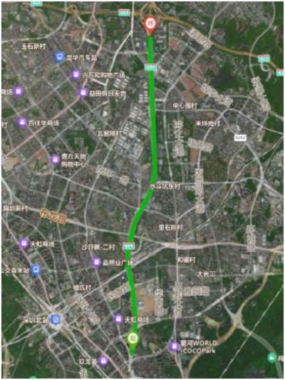
Fig. 1. Experimental section of the Meiguan Expressway (screenshot of a map from open sources)
The study focused on the south-north direction of the Meiguan Expressway. Data was collected using six inductive loop detectors (ILD) installed in the inner and outer pathways.
The following parameters were recorded at 5-minute intervals:
Total data volume: 1,144 records.
To improve the quality of analysis and modeling, preliminary data processing was performed [12]. The following were its stages.
1. Data screening. A selection from a set for identifying data that was valid and relevant to the model. Initially, the source dataset was divided by dates to select records with the most complete data, without obvious gaps. Invalid records with obvious gaps were removed. From the selected dates with complete data, consecutive dates were selected to study temporal variations in the flow.
2. Completing missing data. To provide accurate data collection, the equipment must operate without interruption. This can be hampered by random factors such as malfunctions, vehicle detector failures, weather conditions, power outages, etc. Therefore, the collected data was sometimes incomplete and contained gaps. However, they might contain important information about the process patterns. As a result, the prediction model did not receive sufficient data and became unstable, reducing the prediction reliability. Thus, before building a prediction model, it was required to fill in the missing data.
To compensate for periodically occurring time gaps in the traffic flow data, the presented work used the weighted mean method [13].
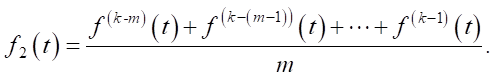
Step 1. Obtaining the mean value of traffic intensity for n points in time preceding the current moment:
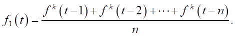
Step 2. Mean traffic intensity at the current moment, for the previous m days:
Step 3. Filling in missing data:
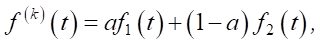
where f(k)(t) — reconstruction of traffic flow data at time t of day k, ɑ — weight coefficient, ɑ = 0.6.
The method is the basic one when working with missing data. It takes into account such properties of traffic volume data as:
3. Normalization. Traffic flow data can vary significantly depending on the time of day, road segment, and other factors, resulting in a wide spread of values. The activation function of some neural nodes takes values in the range [ 0, 1]. Therefore, normalization is performed before training [14]. This eliminates the impact of outliers in the data (samples that deviate significantly from others), and also speeds up network training and improves convergence.
The basic normalization methods are linear, nonlinear, and 0-mean normalization. The activation function takes values from 0 to 1, therefore, this article uses the maximum-minimum linear normalization method to transform traffic flow values into the range [ 0, 1]:
where f — raw traffic flow data; fmin — minimum value in traffic flow data; fmax — maximum value in traffic flow data; f(t) — normalized value of traffic flow.
The processed data were reduced using the inverse normalization formula after the prediction model was derived:
The data sampling frequency was 5 minutes, and the final preprocessed data volume was 3,168 records. Some of these records, obtained on June 17, 2021, are presented in Table 1.
Table 1
Examples of Preprocessed Experimental Data
|
Traffic intensity, units/5 min |
Detector occupancy, % |
Traffic flow speed, km/h |
Time interval, 5 min |
|
258 |
13.93 |
83.62 |
1 |
|
255 |
14.48 |
79.88 |
2 |
|
223 |
12.08 |
82.25 |
3 |
|
340 |
18.39 |
82.04 |
4 |
|
254 |
13.86 |
83.3 |
5 |
|
263 |
13.98 |
84.87 |
6 |
|
231 |
12.49 |
85.89 |
7 |
|
151 |
7.87 |
84.94 |
8 |
|
223 |
11.96 |
83.81 |
9 |
|
226 |
11.95 |
86.92 |
10 |
|
166 |
8.59 |
86.17 |
11 |
|
140 |
7.45 |
83.29 |
12 |
|
143 |
7.85 |
83.99 |
13 |
|
231 |
12.67 |
84.71 |
14 |
|
147 |
7.55 |
89.53 |
15 |
|
96 |
4.90 |
90.74 |
16 |
|
128 |
7.02 |
83.94 |
17 |
|
106 |
5.75 |
81.99 |
18 |
|
128 |
7.24 |
79.4 |
19 |
|
136 |
6.99 |
84.57 |
20 |
Feature extraction is a key step in building an effective traffic flow prediction model. Traffic data analysis and processing provide key feature information, which improves model performance and accuracy.
1. Time-lag feature extraction.
Data from one time series depends on other time series, and the autocorrelation function (ACF) describes the correlation of a time series with different lags, i.e., the degree of linear correlation between the series itself and its own lagged values [15]. This determines the relationship between current and past values. When analyzing time series, the relationship between the current value Yt and its value Yt at some previous point in time is of interest. Period of Lag k is the time interval between the current time point t and k-th time point in the past t-k.
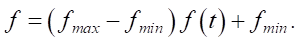
When predicting traffic flows, ACF was used to determine periodicity and trends in time series data. This made it possible to select an appropriate lag step as a feature and reflect the dynamics of changes in traffic flow parameters (Fig. 2).
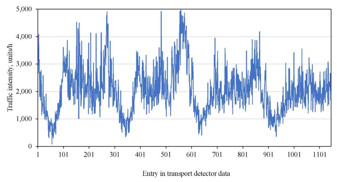
Fig. 2. Traffic dynamics on Meiguan Expressway
For the time series of traffic flow data, the ACF was calculated and the correlation between different time lags (e.g., t-1, t-2, ..., t-n) and the current moment t. The calculation results are presented in Figure 3.
Fig. 3. Autocorrelation coefficients for different lag steps
Using the ACF threshold filtering method, three time lags with an autocorrelation coefficient >0.6 were selected: (Lag 1: 0.70, Lag 2: 0.63, Lag 3: 0.60). These lags were chosen as input features for the model. This approach enhances the model's ability to capture temporal patterns and provides a reliable data base for subsequent prediction models.
2. Interaction of speed and detector occupancy.
The product of speed and detector occupancy is used as a complex metric to represent the spatial-temporal variation of traffic flow [16]. Detector occupancy and speed are important traffic flow metrics. Their product can be used as a “feature interaction” term. This creates a new feature that better reflects the complexity and dynamics of traffic flow. Adding interaction terms can improve the expressiveness and approximation capabilities of machine learning models, specifically those such as LSTM and SVR. Interaction terms provide more information, helping the model better understand patterns and relationships in the data.
Model Architecture and Estimates
This paper evaluates the model prediction performance using the following representative performance metrics:
– mean absolute error;
– mean absolute percentage error;
– root mean square error [21].
This approach allows us:
– to quantitatively evaluate the accuracy of LSTM and SVR models;
– to visualize the discrepancy between actual traffic flow and the prediction results obtained using LSTM.
To test the statistically significant difference between the prediction errors of the LSTM and SVR models, this paper uses the Wilcoxon signed-rank test [22]. This is a nonparametric test for paired data in statistics. It is especially useful for small samples and when the data does not follow a normal distribution. The initial hypothesis (H0) of the test is that there is no significant difference between the prediction errors of the LSTM and SVR models. P-value is a probability value used to detect a significant difference between two related samples. If P is less than a specified significance level (usually 0.05), the null hypothesis is rejected. In this case, it is assumed that the distribution of the difference between the two samples varies, meaning the sum of the ranks is significantly dissimilar. This paper demonstrates a significant difference in the prediction performance of LSTM and SVR. The calculation steps are described below.
Step 1. Calculating the difference in prediction errors between two models. The difference in prediction errors for each observation is calculated using the formula:
Step 2: Calculating the absolute values of the differences and ranking them.
Step 3: Calculating the sums of positive and negative ranks.
Step 4: Calculating the Wilcoxon P and comparing it to the critical value.
Results. In this study, Python was used to preprocess traffic data. The experimental dataset consisted of traffic data from June 17 to 20, 2021 (Table 2). The data was recorded at 5-minute intervals and contained 1,144 records. For traffic flow prediction and model evaluation, the data was divided into training and test sets.
Table 2
Statistical Information about Datasets
|
Indicator |
Traffic intensity (units/h) |
|
Minimum value |
84 |
|
Maximum value |
4968 |
|
Mean value |
2052 |
|
Median |
1944 |
|
Standard Deviation |
864 |
The minimum traffic volume value is 84, and the maximum is 4968, indicating significant data dispersion. This suggests extremely low traffic volumes during certain periods of the day (e.g., early morning) and extremely high traffic volumes during rush hours. The mean value is 2052, and the median is 1944. The fact that the median is slightly smaller than the mean indicates the right-skewed data distribution. This means that traffic volume is high in most time intervals, while some periods of low volume (primarily early morning and late night) reduce the overall mean value. A standard deviation of 864 confirms significant flow fluctuations and sudden changes in traffic volume. Thus, the dataset is suitable for studying long-term dependences and nonlinear characteristics of time series and can serve as an experimental sample for traffic flow prediction.
As noted above, to improve prediction efficiency, this study uses the lag characteristic and the interaction variable between speed and detector occupancy as input features. This allows for a full accounting of the relationships between time series information and flow characteristics.
The SVR method uses the radial basis function (RBF kernel) as a kernel to capture nonlinear relationships.
Key parameters:
1) penalty coefficient C = 2 (tolerable error control);
2) maximum number of iterations — 120.
The LSTM parameters used in this study are described below.
1) Input layer: time step is the feature extraction delay step, which is equal to 1, 2, 3.
2) Hidden layer: single-layer LSTM structure containing 150 cells using the tanh activation function.
3) Regularization: a 10% dropout mechanism used to prevent overfitting.
4) Output Layer: a fully connected layer using a linear activation function to ensure continuous predicted values.
5) Training Strategy: Adam optimizer, learning rate = 0.08, batch size = 128, number of training rounds (epochs) = 120.
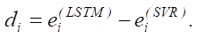
Figures 4 and 5 show the comparison of predicted and true values for the LSTM and SVR models.
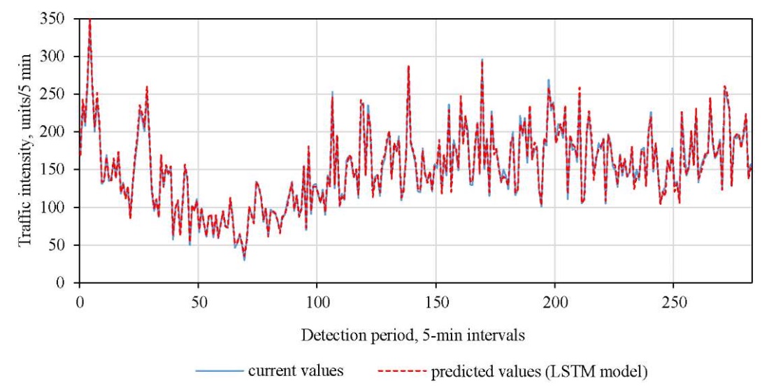
Fig. 4. Comparison of predicted and true values of LSTM
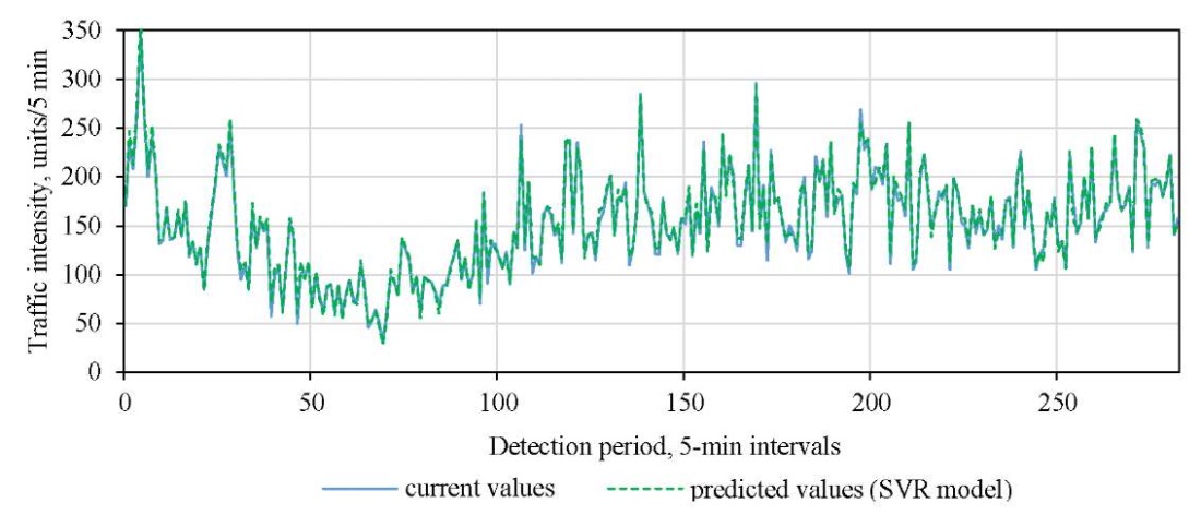
Fig. 5. Comparison of predicted and true values of SVR
The graphs show that the predicted values of the LSTM and SVR models reproduce real traffic flow dynamics well, with a small range of prediction errors. Therefore, these models were selected as control models for further evaluation of the efficiency of various methods in traffic flow prediction.
To increase the reliability of the experimental results and further validate the efficiency of the predictive models, this study conducted 10 training runs with different random initial values. In each experiment, the results for root mean square errors (RMSE), mean absolute errors (MAE), and mean absolute percentage errors (MAPE) were recorded.
To more clearly evaluate predictive performance, RMSE was chosen as the primary metric. From 10 experiments for each model, the five best results were selected, from which average values were calculated for comparative analysis.
Table 3 shows the prediction accuracy of the LSTM and SVR models. The RMSE, MAE, and MAPE errors for the LSTM model were 17.86%, 19.82%, and 25.78% lower, respectively, indicating higher prediction accuracy. MAPE reflects the percentage of prediction error relative to actual values. A lower MAPE score indicates more little relative errors for LSTM at different flow levels. LSTM demonstrates prediction stability during both peak and minimum periods, while SVR is more sensitive to extreme values.
Table 3
Prediction Errors of LSTM and SVR Models
|
Model |
RMSE |
MAE |
MAPE |
|
LSTM |
4.6 |
3.48 |
2.39% |
|
SVR |
5.6 |
4.34 |
3.22% |
Figure 6 shows the absolute percentage error of the predicted values relative to the actual values for each time interval along the flow time series. It is clearly seen that the absolute percentage error of the LSTM model is lower at most time points.
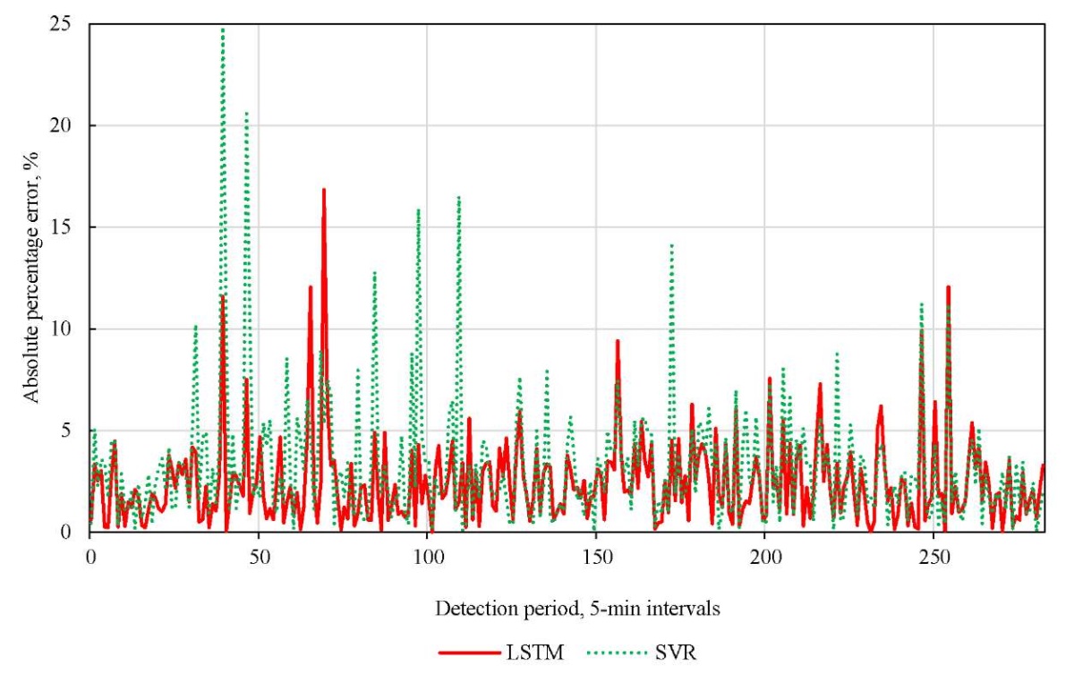
Fig. 6. Absolute percentage error for different time slices of LSTM and SVR
Comparing Figure 6 and Figure 4 (real values) shows that the peaks in the graph with large prediction errors correspond to time intervals with sharp changes in flow intensity. LSTM produces more stable prediction results and outperforms SVR in capturing flow peaks with nonlinear dynamic changes.
From Figure 6, we extracted the time intervals with the greatest error (timeslice: 36–72) and the least error (timeslice: 108–144). The numbers represent the 5-minute intervals. Data from these two periods was used in training models and predicting traffic flow to compare the ability of LSTM and SVR to capture dynamic characteristics of traffic flow. Figure 7 shows the prediction results of the LSTM and SVR models for the two specified time periods compared to the actual values.
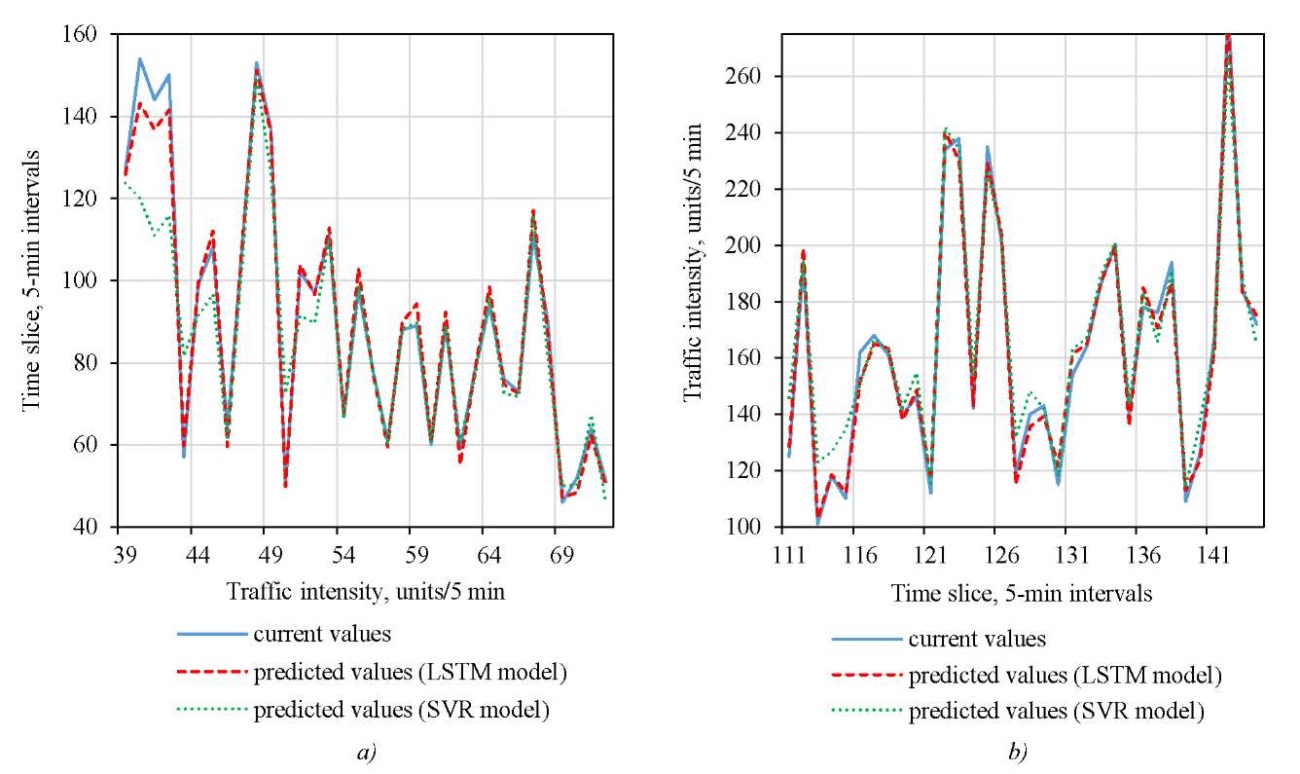
Fig. 7. Prediction curves by time periods:
a — for time slices with the greatest error;
b — for time slices with the least error
Table 4 presents the prediction results of the two models for the periods with the greatest and least errors.
Table 4
Data on the Least and Greatest Prediction Errors of LSTM and SVR
|
Period |
Model |
RMSE |
MAE |
MAPE |
|
With the least error |
LSTM |
6.14 |
4.84 |
2.99% |
|
SVR |
9.67 |
7.37 |
5.19% |
|
|
With the greatest error |
LSTM |
3.32 |
2.57 |
2.88% |
|
SVR |
12,39 |
7.43 |
8.09% |
The comparison shows that LSTM demonstrates better accuracy in periods with the least flow rate prediction error: the RMSE, MAE, and MAPE errors for the LSTM model are 36.5%, 34.3%, and 42.3% lower, respectively. In periods with the greatest flow rate prediction error, the advantage of LSTM is particularly noticeable: the RMSE, MAE, and MAPE errors for the LSTM model are 73.2%, 65.4%, and 64.4% lower, respectively. This shows the higher adaptability of this model.
To statistically test the significance of differences between the models, the Wilcoxon signed-rank test is used. The result (P = 2.44e-15) is tangibly less than 0.05. Therefore, the null hypothesis of no difference in prediction errors should be rejected. This proves a statistically significant difference in the performance of the models.
Along with RMSE, MAE, and MAPE evaluation, it is confirmed that the LSTM error is significantly lower and the error distribution is more concentrated, indicating higher prediction stability. The results convincingly demonstrate the advantages of LSTM when working with traffic flow time series data.
Discussion. Thus, prediction quality depends on the model architecture. Combining interaction variables and lag metrics in the LSTM structure resulted in improved prediction accuracy. Experiments revealed that LSTM outperformed SVR in terms of root-mean-square, mean absolute, and mean absolute percentage errors. This confirmed its superior predictive power under various traffic flow conditions. Flow stability affected prediction accuracy, but LSTM, thanks to its superior time series modeling capabilities, was able to more effectively account for flow temporal dependences and maintain high accuracy even under significant fluctuations. It is worth noting that LSTM not only effectively accounted for traffic flow temporal dependences but also adapted to complex, long-term dynamic changes. Hence — the more accurate results of short-term prediction.
The advantages of LSTM were significantly more pronounced in periods with the greatest flow rate prediction errors. The gain of this model in absolute percentage error in periods with the least error reached 42.3%, while in periods with the greatest error, it was 64.4%. For RMSE and MAE, the difference was twofold or almost twofold. The RMSE figures were 36.5% (periods with the least error) and 73.2% (periods with the greatest error). The corresponding figures for MAE were 34.3% and 65.4%.
The SVR method adapts well to nonlinear characteristics of traffic flow data, it is robust to outliers, and can adapt to various data characteristics through adjusting the kernel function and regularization parameters. Its computational efficiency is higher. However, this model is more sensitive to data noise due to the complexity of modeling long-term time dependence, which reduces prediction stability, especially in the presence of dynamic traffic flow fluctuations with great errors. The predictive performance of SVR is limited by its weaker, nonlinear approximation ability to sudden flow changes due to limitations of its own architecture, resulting in a significant increase in errors.
Conclusion. This study compared the performance of long short-term memory (LSTM) networks and support vector machine regression (SVR) for short-term traffic flow prediction on the Meiguan Expressway in Shenzhen. The LSTM model performed 17.86% better than the SVR in terms of mean squared error, 19.82% better in terms of mean absolute error, and 25.78% better in terms of mean absolute percentage error.
LSTM is also supported by its higher accuracy in periods with both the least error and the greatest one. In the first case, compared to SVR, the LSTM errors were 34.3–42.3% lower, in the second — by 64.4–73.2 %.
Thus, when choosing between a neural network and a machine learning model for short-term traffic flow prediction on a highway, the neural network model, in this case LSTM, should be preferred.
Let us outline three major results of this study for solving the problem of high-quality short-term prediction of traffic flows in large cities.
Short-term traffic flow prediction based on LSTM allows for relatively accurate traffic volume prediction. This can serve as a basis for optimizing traffic management strategies, reducing congestion and pollutant emissions, and optimizing intelligent transportation systems.
A promising area for further research is the development of hybrid architectures that integrate contextual data (e.g., weather conditions, traffic incidents, or infrastructure features). This will improve the reliability and robustness of real-time prediction.
1. Сhina Statistical Yearbook 2023. URL: https://www.stats.gov.cn/sj/ndsj/2023/indexeh.htm (accessed: 06.10.2024).
2. Sustainable Development Goals. United Nations. (In Russ. URL: https://www.un.org/sustainabledevelopment/ru/sustainable-development-goals/ (accessed: 21.10.2025).
1. Garg T, Kaur G. A Systematic Review on Intelligent Transport Systems. Journal of Computational and Cognitive Engineering. 2022;2(3):175–188. https://doi.org/10.47852/bonviewJCCE2202245
2. Vlahogianni EI, Matthew GK, Golias JC. Short-Term Traffic Forecasting: Where We Are and Where We’re Going. Transportation Research. Part C: Emerging Technologies. 2014;43(1):3–19. https://doi.org/10.1016/j.trc.2014.01.005
3. Williams BM, Hoel LA. Modeling and Forecasting Vehicular Traffic Flow as a Seasonal ARIMA Process: Theoretical Basis and Empirical Results. Journal of Transportation Engineering. 2003;129(6):664–672. https://doi.org/10.1061/(ASCE)0733-947X(2003)129:6(664)
4. Lippi M, Bertini M, Frasconi P. Short-Term Traffic Flow Forecasting: An Experimental Comparison of Time-Series Analysis and Supervised Learning. IEEE Transactions on Intelligent Transportation Systems. 2013;14(2):871–882. https://doi.org/10.1109/TITS.2013.2247040
5. Zhenjin Huang, Hao Ouyang, Yiming Tian. Short-Term Traffic Flow Combined Forecasting Based on Nonparametric Regression. In: Proc. International Conference of Information Technology, Computer Engineering and Management Sciences. New York City: IEEE; 2011. P. 316–319. https://doi.org/10.1109/ICM.2011.89
6. Polson NG, Sokolov VO. Deep Learning for Short-Term Traffic Flow Prediction. Transportation Research. Part C: Emerging Technologies. 2017;79:1–17. https://doi.org/10.1016/j.trc.2017.02.024
7. Ceperic E, Ceperic V, Baric A. A Strategy for Short-Term Load Forecasting by Support Vector Regression Machines. IEEE Transactions on Power Systems. 2013;28(4):4356–4364. https://doi.org/10.1109/TPWRS.2013.2269803
8. Weiwei Zhu, Jinglin Wu, Ting Fu, Junhua Wang, Jie Zhang, Qiangqiang Shangguan. Dynamic Prediction of Traffic Incident Duration on Urban Expressways: A Deep Learning Approach Based on LSTM and MLP. Journal of Intelligent and Connected Vehicles. 2021;4(2):80–91. https://doi.org/10.1108/JICV-03-2021-0004
9. Peng Chen, Yong-zai Lu. Extremal Optimization for Optimizing Kernel Function and Its Parameters in Support Vector Regression. Journal of Zhejiang University Science C. 2011;12:297–306. https://doi.org/10.1631/jzus.C1000110
10. Feihu Ma, Shiqi Deng, Sang Mei. A Short-Term Highway Traffic Flow Forecasting Model Based on CNN-LSTM with an Attention Mechanism. Journal of Physics: Conference Series. 2023;2491:012008. https://doi.org/10.1088/1742-6596/2491/1/012008
11. Liu Mingyu, Wu Jianping, Wang Yubo, He Lei. Traffic Flow Prediction Based on Deep Learning. Journal of System Simulation. 2018;30(11):4100–4106. URL: https://dc-china-simulation.researchcommons.org/journal/vol30/iss11/7 (accessed 09.09.2025).
12. García S, Ramírez-Gallego S, Luengo J, Benítez JM, Herrera F. Big Data Preprocessing: Methods and Prospects. Big Data Analytics. 2016;1:9. https://doi.org/10.1186/s41044-016-0014-0
13. Robin Kuok Cheong Chan, Joanne Mun-Yee Lim, Rajendran Parthiban. A Neural Network Approach for Traffic Prediction and Routing with Missing Data Imputation for Intelligent Transportation System. Expert Systems with Applications. 2021;171:114573. https://doi.org/10.1016/j.eswa.2021.114573
14. Chahinez Ounoughi, Sadok Ben Yahia. Sequence to Sequence Hybrid Bi-LSTM Model for Traffic Speed Prediction. Expert Systems with Applications. 2024;236:121325. https://doi.org/10.1016/j.eswa.2023.121325
15. Rong Chen, Lijian Yang, Christian Hafner. Nonparametric Multistep-Ahead Prediction in Time Series Analysis. Journal of the Royal Statistical Society. Series B: Statistical Methodology. 2004;66(3):669–686. https://doi.org/10.1111/j.1467-9868.2004.04664.x
16. Aqib M, Mehmood R, Alzahrani A, Katib I, Albeshri A, Altowaijri SM. Smarter Traffic Prediction Using Big Data, In-Memory Computing, Deep Learning and GPUs. Sensors. 2019;19(9):2206. https://doi.org/10.3390/s19092206
17. Xianyao Ling, Xinxin Feng, Zhonghui Chen, Yiwen Xu, Haifeng Zheng. Short-Term Traffic Flow Prediction with Optimized Multi-kernel Support Vector Machine. In: Proc. IEEE Congress on Evolutionary Computation (CEC). New York City: IEEE; 2017. P. 294–300. https://doi.org/10.1109/CEC.2017.7969326
18. Zhou Zhao, Ashok Srivastava, Lu Peng, Qing Chen. Long Short-Term Memory Network Design for Analog Computing. ACM Journal on Emerging Technologies in Computing Systems (JETC). 2019;15(1):1–27. https://doi.org/10.1145/3289393
19. Srivastava N, Hinton G, Krizhevsky A, Sutskever I, Salakhutdinov R. Dropout: A Simple Way to Prevent Neural Networks from Overfitting. Journal of Machine Learning Research. 2014;15:1929–1958. URL: https://www.jmlr.org/papers/volume15/srivastava14a/srivastava14a.pdf?utm_content=buffer79b4 (accessed: 21.10.2025).
20. Yang Zhu, Yijun Gao, Zhenhao Wang, Guansen Cao, Renjie Wang, Song Lu, et al. A Tailings Dam Long-Term Deformation Prediction Method Based on Empirical Mode Decomposition and LSTM Model Combined with Attention Mechanism. Water. 2022;14(8):1229. https://doi.org/10.3390/w14081229
21. Pan B, Demiryurek U, Shahabi C. Utilizing Real-World Transportation Data for Accurate Traffic Prediction. In: Proc. IEEE 12th International Conference on Data Mining. New York City: IEEE; 2012. P. 595–604. https://doi.org/10.1109/ICDM.2012.52
22. Moors G, Vriens I, Gelissen JP, Vermunt JK. Two of a Kind. Similarities Between Ranking and Rating Data in Measuring Values. Survey Research Methods. 2016;10(1):15–33. https://doi.org/10.18148/srm/2016.v10i1.6209.
Ivan V. Topilin, Cand.Sci. (Eng.), Associate Professor of the Department of Organization of Transportation and Road Traffic Management
1, Gagarin Sq., Rostov-on-Don, 344003
Scopus Author ID: 57193746467
Mengyi Han, Postgraduate student of the Department of Organization of Transportation and Road Traffic Management
1, Gagarin Sq., Rostov-on-Don, 344003
Anastasia A. Feofilova, Cand.Sci. (Eng.), Associate Professor of the Department of Organization of Transportation and Road Traffic Management
1, Gagarin Sq., Rostov-on-Don, 344003
Scopus Author ID: 57193742031
Nikita A. Beskopylny, Postgraduate student of the Department of Organization of Transportation and Road Traffic Management
1, Gagarin Sq., Rostov-on-Don, 344003
Scopus ID: 57221328153
When choosing between a neural network and a classical machine learning model for short-term traffic flow forecasting on a highway, preference should be given to a neural network architecture — specifically, LSTM. It is shown that a model with long short-term memory produces more accurate prediction. Its architecture better captures the temporal structure and complex dynamics of traffic. The support vector machine produces higher errors during sudden changes in flow. The results can be applied to reducing congestion and emissions on highways. The approach is useful for the development of intelligent transportation systems in cities.
Topilin I.V., Han M., Feofilova A.A., Beskopylny N.A. Comparative Analysis of Neural Network and Machine Learning Models for Short-Term Traffic Flow Prediction on Shenzhen Expressway. Advanced Engineering Research (Rostov-on-Don). 2025;25(4):350-362. https://doi.org/10.23947/2687-1653-2025-25-4-2215. EDN: DWKVUM


Advanced Engineering Research (Rostov-on-Don)
ISSN 2687-1653 (Online)
Contact with: Publisher / Editorial Office of the Journal
Publisher: Don State Technical University - DSTU, Rostov-on-Don, Russia - https://donstu.ru/en/
Editor-in-Chief: Alexey N. Beskopylny, Dr.Sci. (Eng.), Professor, Vice-Rector, Don State Technical University (Rostov-on-Don, Russia)
Don State Technical University
1, Gagarin Sq., Rostov-on-Don, 344003, Russia
tel.: +7 (863) 2738-372, e-mail: vestnik@donstu.ru
16+
Processing of personal data