Contents
Scroll to:
https://doi.org/10.23947/2687-1653-2025-25-4-2206
EDN: VHVNIF
Scroll to:
Introduction. Modern trends in construction, related to the optimization of weight and materials, require accurate methods for calculating the stress-strain state, particularly of beams with variable stiffness. Analytical calculation of the stressstrain state for such beams is fraught with considerable difficulties, limiting its practical application. Numerical methods, specifically the Finite Element Method (FEM), are widely used to solve these problems, where the law of stiffness change is typically approximated by a piecewise (discrete) function. This study is aimed at the development of an approach based on piecewise-linear approximation of stiffness. Linear stiffness approximation suggests an optimal balance of accuracy and computational resources. This approach provides significantly higher accuracy compared to the traditional discrete approximation with similar computational complexity, allowing for adequate modeling of both smooth stiffness gradients and its violent changes.
Materials and Methods. A first-approximation stiffness matrix for a one-dimensional beam finite element with linearly varying flexural stiffness was derived on the basis of a variational formulation of the problem. An exact stiffness matrix was obtained by direct integration of the differential equation for beam bending. In the calculation examples, an exact solution was obtained using the Maple software package. The numerical solution using FEM was implemented in the author's program written in Python.
Results. During the study, approximate and exact stiffness matrices of the beam finite element were obtained, as well as the vector of nodal reactions (loads) from distributed loads. The efficiency of the proposed approach was demonstrated by numerical examples. The results obtained by the FEM were verified using analytical calculations. Based on the performed calculations, recommendations and criteria for using the exact or approximate stiffness matrix were developed.
Discussion. Finite elements that account for linear change of stiffness along the length make it possible to increase the accuracy of the results and reduce the degree of discretization of the computational scheme by more than two times. The approximate matrix shows good convergence with a smooth change in stiffness along the length. In such cases, discrete approximation is also acceptable. The exact matrix allows for calculating cases where the stiffness within the beam changes by orders of magnitude with low error. The classical discrete approximation in this case does not ensure high accuracy of the calculation results.
Conclusion. The paper presents stiffness matrices for finite elements that account for linear change of stiffness along the length. Their derivation is performed by two methods: on the basis of a variational formulation of the problem, and by direct integration of the differential equation of bending. The resulting matrices enable more accurate stress-strain analysis of beams with variable stiffness. They have an analytical format that simplifies their integration into existing software systems. Further research will be directed towards applying the obtained matrices to the calculation of reinforced concrete beams, considering physical nonlinearity, as well as to solving problems of stability and dynamics of beams with variable stiffness.
Tsybin N.Yu. Exact and Approximate Stiffness Matrix and Nodal Load Vector for a Beam Finite Element with Linearly Varying Stiffness along Its Length. Advanced Engineering Research (Rostov-on-Don). 2025;25(4):275-289. https://doi.org/10.23947/2687-1653-2025-25-4-2206. EDN: VHVNIF
Introduction. In modern engineering practice, specifically in the context of sustainable development and resource optimization, structures with variable stiffness — for example, beams with variable cross-sections — are widely used [1]. Such solutions significantly reduce the material consumption and dead weight of structures, which directly improves their cost-effectiveness and environmental friendliness by reducing material consumption [2]. In addition, the mathematical model of a beam of variable stiffness serves as a tool for the qualitative description of the stress-strain state of reinforced concrete elements, in which the change in stiffness occurs due to the nonlinear behavior of the material [3][4] and the formation of cracks [5][6].
In statically indeterminate beams, which are common in structural mechanics, the distribution of internal forces depends on the stiffness ratio of the elements. Neglecting the variable nature of stiffness can cause significant errors in determining internal forces and, consequently, the incorrect cross-section selection, which compromises both the reliability and economic viability of the project. Figure 1 shows a clear example: taking into account variable stiffness in a beam (Fig. 1 b) has led to a radical change in the bending moment diagram compared to the calculation model of constant stiffness (Fig. 1 a).
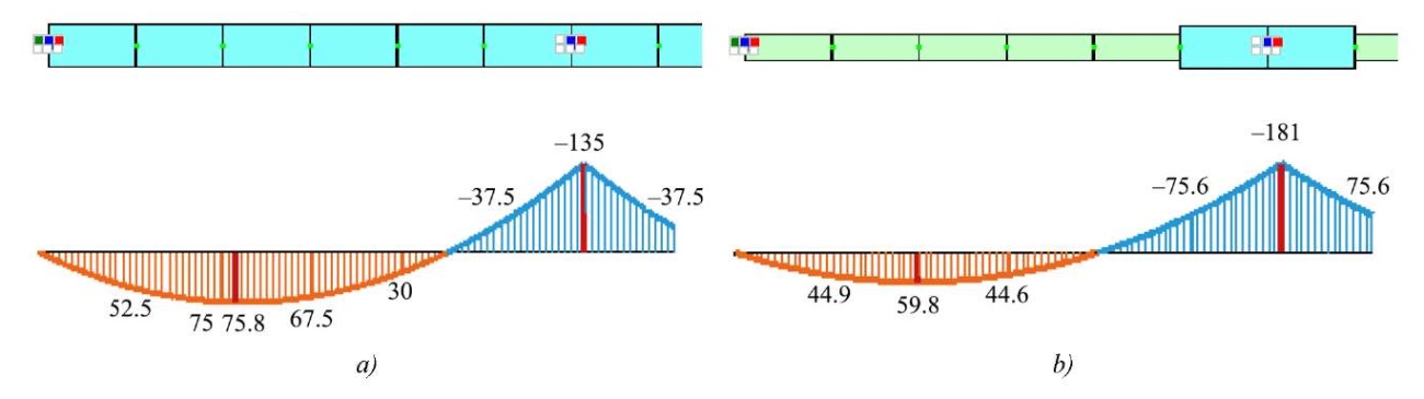
Fig. 1. Results of calculation of statically indeterminate beam:
a — fragment of statically indeterminate beam of constant stiffness and diagram of bending moments in it;
b — the same for beam of variable stiffness
The analysis of beams with variable cross-sections is traditionally performed using numerical methods, in particular, the finite element method (FEM). Despite the existence of analytical solutions [7], they are often represented as complex series [8] or special functions [9], which complicates their practical implementation in engineering software. Moreover, such solutions often lack universality for arbitrary laws of stiffness change and boundary conditions [10][11].
The stress-strain state of beams with variable cross-sections has been studied by various authors for a long time. In the context of numerical calculations using FEM, some of the first works [12][13] can be mentioned. The most common approach to accounting for variable stiffness is a discrete approximation using finite elements of constant stiffness (Fig. 1 b), whose value is taken equal to the average in the section [14][15]. Despite its simplicity, this approach does not always ensure the required accuracy of calculations.
More accurate results are obtained by using a linear approximation of the stiffness within the finite element. This approach is described in this article. At the same time, classical methods for constructing stiffness matrices for elements with variable parameters [16], based on variational approaches [17] or approximations [18], may not provide the exact fulfillment of the differential equations of equilibrium and boundary conditions. This causes errors with significant changes in stiffness along the length of the element or in extreme cases, for example, when modeling zones with a sharp drop in stiffness (formation of cracks, plastic hinge).
Thus, the relevance of this study is determined by the need to develop an efficient and more accurate method for calculating beams with variable stiffness.
The objective of this study is to obtain and verify stiffness matrices for a beam finite element with a piecewise linear law of stiffness change.
To reach this objective, the following tasks were formulated:
Materials and Methods
Variational Method for Obtaining the Stiffness Matrix. Variational methods [19] are the generally accepted and most versatile methods for obtaining the stiffness matrix of a finite element. The accuracy of the resulting matrix depends on how well the input approximation of the desired function reflects the solution to the differential equation.
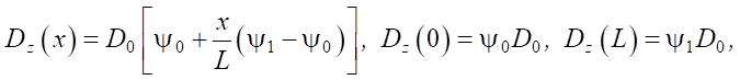
For the beam under consideration, the classical Euler-Bernoulli hypotheses are applied. The change in the flexural stiffness of the cross-section Dz along the length of the finite element is assumed to be a linear function:
 (1)
(1)
where D0 — initial stiffness; L — length of the finite element; ψ0 and ψ1 — coefficients that take into account the change in initial stiffness D0 at the beginning and end of the element, respectively. In this case, ψ0 ≥ 0 and ψ1 ≥ 0.
The finite element method is considered in the form of displacements. The unknowns are the deflection and rotation angle of the section vi and φi (Fig. 2 a) at the beginning x = 0 and end x = L of the element.
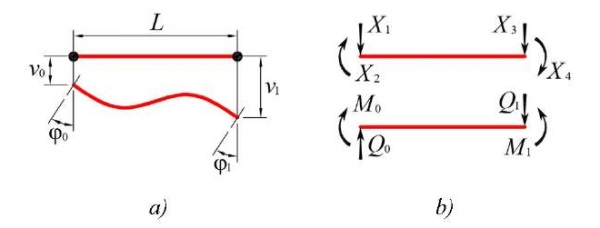
Fig. 2. Beam finite element:
a — unknowns of the finite element method;
b — nodal loads and internal forces
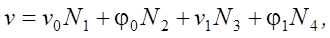
To approximate the displacement function v(x), Hermite polynomials are used [1][4]:
 (2)
(2)
where Ni — shape functions (Hermite polynomials) written below:
 (3)
(3)
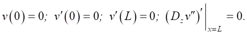
Approximation (2) corresponds to the following boundary conditions:
 (4)
(4)
The prime in (4) denotes the derivative of function v(x) in respect to x.
From formulas (3), it follows that classical shape functions do not take into account the distribution of bending stiffness along the length of the element, which, in turn, negatively impacts the accuracy of the calculation results. To improve the accuracy of calculations, when using a variational formulation of the problem, the double approximation method can be applied [20].
The bending moment is associated with the curvature by the relation:
 (5)
(5)
Here, Dz — bending stiffness of the beam cross-section according to (1).
Taking into account (2) and (3):
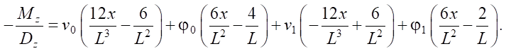 (6)
(6)
The potential energy of bending deformation is determined by the formula:
 (7)
(7)
Taking into account (6) and (1), formula (7) takes the form:
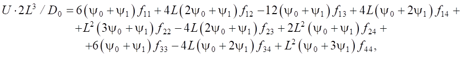 (8)
(8)
where
 (9)
(9)
If we introduce the vector of unknowns 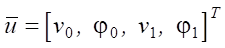 , then (8) can be rewritten in the following form:
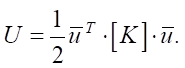 (10)
(10)
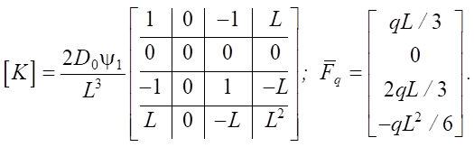
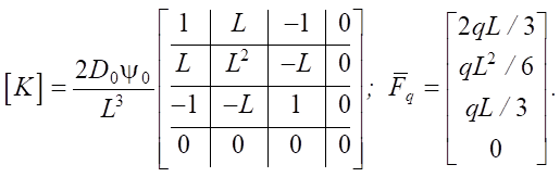
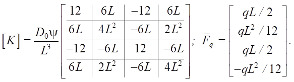
Here, [K] — stiffness matrix of the element, determined taking into account (8) and (9):
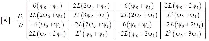 (11)
(11)
This case ψ0 = ψ0 = 1 corresponds to the classical beam stiffness matrix.
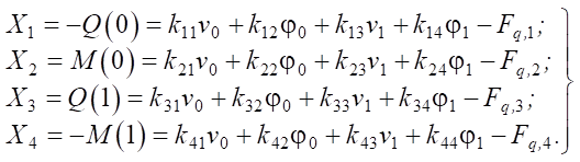
The positive directions of the nodal loads and internal forces are shown in Figure 2 b, from which it follows:
 (12)
(12)
Let us calculate the work of external forces.
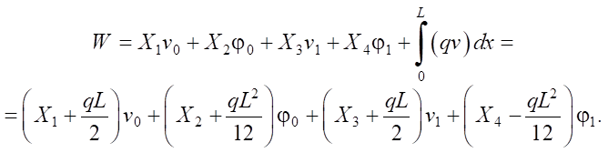 (13)
(13)
In matrix form
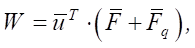 (14)
(14)
where  — vector of concentrated nodal loads;
  — vector of nodal loads from distributed loads. The components of these vectors have the form (15):
 (15)
(15)
As we can see, the vector of nodal forces from distributed loads obtained in (15) does not take into account the change in stiffness along the length. This is a drawback of the variational approach in the context of the problem under consideration.
The total energy of the system, taking into account (10) and (14), is determined by the expression:
 (16)
(16)
Applying the principle of minimum potential energy, we obtain the condition for the stationarity of functional (16):
 (17)
(17)
The basic equation of the finite element method follows from (17):
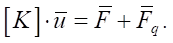 (18)
(18)
Direct Method for Obtaining the Stiffness Matrix. The resulting stiffness matrix (11) has a significant drawback. If we assume v0 = φ0 = 0, as well as ψ0 = 0 and ψ1 = 1 (which corresponds to zero stiffness at the left clamped edge), the moment at the left edge will be determined by the formula:
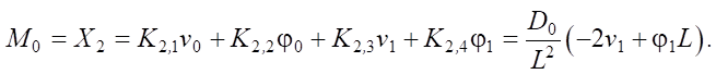 (19)
(19)
Note that (19) considers a limiting case — a mathematical idealization, where the stiffness at the support is not simply small but asymptotically tends to zero. Thus, in accordance with (19), the moment at the left edge does not vanish, which contradicts formula (5). The reason lies in the inaccurate approximation of the deflection function by formula (2). To eliminate this discrepancy, an exact stiffness matrix was found through direct integrating the differential equation for beam bending, taking into account the change in stiffness along the length by formula (1).
A similar approach was used by other authors. In [21], the solution is obtained in the form of power series, therefore, it cannot be considered closed. In [22], a direct integration method is used to obtain the stiffness matrix of an element with a power law of stiffness change for stability problems. In [23], an arbitrary law of stiffness change along the length is considered. However, for the practical use of the presented results, integration is required. Works [24][25] are devoted to solving stability problems. In these papers, the law of stiffness change along the length is given in the form of a polynomial of the second and fourth degree, while the vector of nodal forces from distributed loads is not provided. A common drawback of works that take into account second and higher order polynomials in the function of stiffness change along the length is the complexity of calculating the stiffness matrix. For example, according to [26], to obtain the stiffness matrix coefficients, it is required to calculate expressions of the form sin[ε ln (λ)] (the original notations are preserved), which complicates the analysis of limiting cases and the implementation of solutions in commercial software packages.
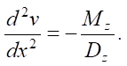
To obtain an accurate stiffness matrix, the differential equation for plane transverse bending of a beam with variable stiffness, known from the course on strength of materials, is considered:
 (20)
(20)
Given the form (1), the general solution to the homogeneous equation (20) will contain a logarithm. We eliminate the dimensional quantities under the logarithm sign by replacing the variable using the formula:
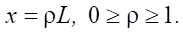 (21)
(21)
Considering (21):
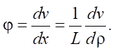 (22)
(22)
As a result, general solution [27] of equation (20) takes the form:
 (23)
(23)
where α = ψ0 / (ψ0 – ψ1), v* — particular solution to the inhomogeneous equation. Due to its cumbersome nature, the particular solution is not given.
Solution (23) is valid for the cases ψ0 ≠ ψ1, ρ ≠ α, since these cases generate uncertainties that are resolved through limiting in formulas (31), (32) and (33).
The unknown integration constants are determined from the boundary conditions:
 (24)
(24)
In (24), the prime denotes the derivative with respect to ρ. Multiplier L at the rotation angles in the boundary conditions (24) is present due to the introduced change of variable (21), which is reflected in (22). After determining the integration constants from (24), the moment and shear force in the beam, taking into account the introduced change of variables, are calculated using the formulas:
 (25)
(25)
The coefficients of the stiffness matrix, taking into account (25) and (12), can be found from the expressions:
 . (26)
Matrix form (26) is equivalent to the one obtained earlier (18). The stiffness matrix in the case under consideration will take the form:
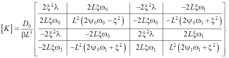 (27)
(27)
In (27), the following notations are introduced for the sake of compactness:
 (28)
(28)
To implement the proposed stiffness matrix in software, it is critical to be able to transform distributed loads into a nodal force vector. The exact expressions for vector are given below.
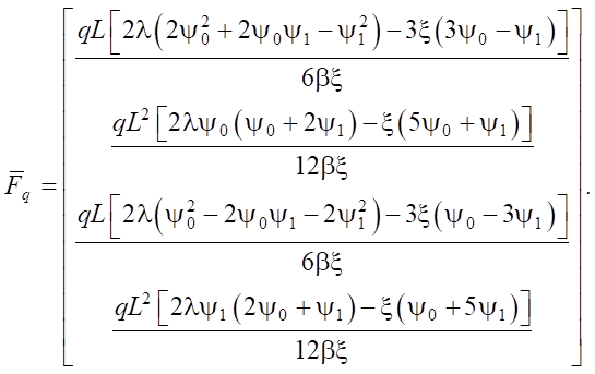 (29)
(29)
The main advantage of the obtained matrix (27) and vector (29) is the simplicity of implementation, as well as the absence of series and special functions in the calculations.
When solving certain problems, it is more convenient to relate section stiffness coefficients ψ0 and ψ1 to the curvature. In this case, it is necessary to know how the curvature is related to the displacements and rotation angles of the nodes of the element. Formula (5) can be used for this. Knowing how the moment is expressed at the beginning and end of the element according to formulas (26), we obtain:
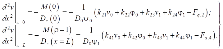 (30)
(30)
Cases ψ0 = 0, ψ1 = 0 and ψ0 = ψ1 = ψ generate uncertainties of various types in matrix (27) and vector (29). Let us develop them.
Case ψ0 = 0.
 (31)
(31)
Case ψ1 = 0.
 (32)
(32)
From (31) and (32), it is evident that the columns and rows of the stiffness matrix, as well as the components of the nodal force vector from distributed loads associated with the bending moments at the left and right ends of the finite element, respectively, are set to zero — which corresponds to equation (5). The vanishing of the bending stiffness can occur, for example, when tensile reinforcement breaks, or the compressed zone of a reinforced concrete beam fails in any section. In the case of a statically indeterminate beam, the structure can continue to function during such failures. In commercial software packages, when such situations arise, hinges are typically activated in the calculation model.
Case ψ0 = ψ1 = ψ. This case corresponds to the classical stiffness matrix.
 (33)
(33)
In practical calculations, to reduce computational errors that may accumulate during the calculation of the stiffness matrix components and factors (28), it is recommended to use formulas (31), (32) and (33) not when strictly reaching the limiting case, but when approaching it. For example, set the threshold conditions for using (27) and (29) in the form ψi > 10⁻⁴ and |1 – ψ0 / ψ1| > 10⁻³. The specified values are approximate and depend on the specific implementation features.
Figure 3 shows graphs of three elements of the stiffness matrix, calculated using formulas (11) and (27) for ψ1 = D0 = L = 1.

Fig. 3. Dependences k11, k22 and k12 on ψ0. Solid lines are based on exact stiffness matrix (27); dashed lines — on approximate matrix (11)
The results presented in Figure 3 show that, for ψ0 = 0 and the corresponding boundary conditions, the stiffness matrix coefficients associated with the moment at the left edge vanish in the exact matrix (27) — this corresponds to the physical meaning. Approximate stiffness matrix (11) does not have this property. With a significant difference in stiffness, at the beginning and end of the element (ψ0 / ψ1 < 0.2), values of the coefficients of the exact and approximate matrices can differ by up to 100% (excluding from consideration the limiting case ψ0 → 0). In such situations, it is recommended to use exact stiffness matrix (27). Similar conclusions can be drawn for the right edge of the finite element.
Research Results. To demonstrate the results obtained using the proposed stiffness matrices, calculation examples are performed for beams of length 2L, shown in Figure 4.
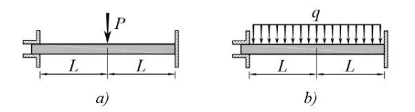
Fig. 4. Schematic diagrams for calculation examples:
a — clamped beam of length 2L, loaded with concentrated force;
b — the same under uniformly distributed load
Due to symmetry with respect to x = L, half of the beam is considered in the solution. The boundary conditions under the action of a concentrated force (diagram in Fig. 4 a) are as follows:
 (34)
(34)
Similarly for the case of distributed load (diagram in Fig. 4 b):
 (35)
(35)
The following stiffness distribution function along the beam length is considered:
 (36)
(36)
s0 and s1 — beam stiffness coefficients at the beginning and middle of the span, that is, Dz(0) = D0s0 and Dz(L) = D0s1. In this case, Dz(L / 2) = D0. It is important to note that (36) determines the law of stiffness change along the length of the beam as a whole, while (1) — along the length of the finite element.
Function (36) is selected on the base of the method of load application and the boundary conditions. In this case, for a beam of constant stiffness, the moments at the support and in the middle of the beam reach maximum values. If the beam material is reinforced concrete, cracks and a decrease in flexural stiffness should be expected at these points [27]. At a quarter span, the moments are close to zero and, consequently, the stiffness is close to the initial Dz(L / 2) = D0.
Figure 5 shows the graphs of the stiffness distribution along the length of the beam, as well as the approximation methods under consideration for two alternatives: option 1 — s0 = 0.001, s1 = 1.0; option 2 — s0 = 0.6, s1 = 0.2.
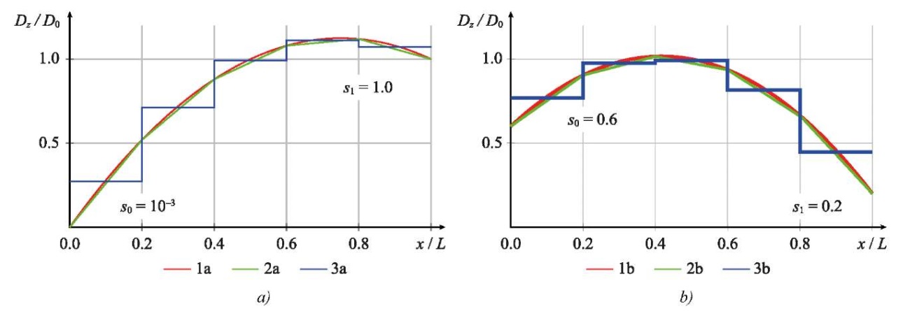
Fig. 5. Stiffness Dz(x) / D0 distribution along the beam length:
a — option 1 — s0 = 0.001 and s1 = 1.0;
b — option 2 — s0 = 0.6 and s1 = 0.2.
Curves 1 a, 1 b — initial function;
2 a, 2 b — piecewise linear approximation;
3 a, 3 b — discrete approximation
From the results presented in Figure 5, it is evident that the linear approximation, even with five finite elements, provides satisfactory agreement (the deviation does not exceed 5%) with the initial function of stiffness change along the length for the examples under consideration. High accuracy is maintained when approximating the stiffness with a piecewise linear function for variable cross-sections of complex shape [28]. The value of the average stiffness for discrete approximation was calculated using the formula:
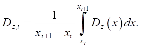 (37)
(37)
The results of calculating the coefficients for the stiffness matrices of finite elements are given in Table 1. For discrete approximation, ψ0 = ψ1 = ψ.
Table 1
Coefficients of Element Stiffness Matrices
|
Element |
1 |
2 |
3 |
4 |
5 |
|||||||||
|
xi |
xi+1 |
0.0 |
0.6 |
0.6 |
1.2 |
1.2 |
1.8 |
1.8 |
2.4 |
2.4 |
3.0 |
|||
|
Option 1: s0 = 0.001 and s1 = 1.0 |
||||||||||||||
|
Coeff. ψ0,1 |
ψ0 |
ψ1 |
ψ0 |
ψ1 |
ψ0 |
ψ1 |
ψ0 |
ψ1 |
ψ0 |
ψ1 |
||||
|
Linear |
0.001 |
0.52 |
0.52 |
0.88 |
0.88 |
1.08 |
1.08 |
1.12 |
1.12 |
1.0 |
||||
|
Discrete |
0.274 |
0.714 |
0.993 |
1.113 |
1.073 |
|||||||||
|
Option 2: s0 = 0.6 and s1 = 0.2 |
||||||||||||||
|
Coeff. ψ0,1 |
ψ0 |
ψ1 |
ψ0 |
ψ1 |
ψ0 |
ψ1 |
ψ0 |
ψ1 |
ψ0 |
ψ1 |
||||
|
Linear |
0.6 |
0.904 |
0.904 |
1.016 |
1.016 |
0.936 |
0.936 |
0.664 |
0.664 |
0.2 |
||||
|
Discrete |
0.768 |
0.976 |
0.992 |
0.816 |
0.448 |
|||||||||
Since an elastic problem is being solved, the results of calculating the stress-strain state components depend linearly on the load magnitude and initial stiffness D0. Therefore, in the calculation, these quantities are assumed to be equal to unity.
The solution to equation (20) with boundary conditions (34) and the law of stiffness change (36) is found analytically for values s0 and s1 under consideration. Due to its cumbersome nature, this solution is not presented here. It was not possible to obtain an analytical solution for arbitrary values s0 and s1.
The results from the obtained analytical solution were then compared to the results of the finite element calculation. In the basic calculation, the beam was divided into five finite elements. To study the effect of the number of finite elements on the accuracy of the results, a series of calculations were performed in which their number varied.
Based on the calculation results, the error value was determined in comparison with the analytical solution. To formulate conclusions regarding the required number of elements, a 5% error threshold was adopted. Conclusions regarding the feasibility of applying this approach in practical calculations were based on the assumption that the threshold accuracy was achieved with fewer than 60 elements — in this case, the finite element length was 50 mm. Using a finer granularity is impractical for calculating beams in building structures — it significantly increases computational costs and calculation time. The maximum number of elements in the calculation examples was set to 400 (with a finite element length of 7.5 mm). With a larger number of finite elements, the solver implemented by the author began to accumulate computational errors.
Example 1. Solution to the problem of bending of a clamped beam loaded at the center with a concentrated force. A sketch of the calculation scheme is shown in Figure 4 a. The stiffness distribution is adopted according to option 1: s0 = 0.001 and s1 = 1. The graph of the stiffness function for this option is shown in Figure 5 a. Figures 6 and 7 show the results of calculating the deflections and bending moments, as well as the calculation error.
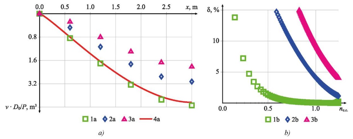
Fig. 6. Results of deflection calculations for the example:
a — calculation results of deflection v depending on x;
b — calculation error depending on the number of finite elements.
1 a, 1 b — linear approximation and exact stiffness matrix (27);
2 a, 2 b — linear approximation and approximate stiffness matrix (11);
3 a, 3 b — discrete approximation;
4 a — analytical calculation results
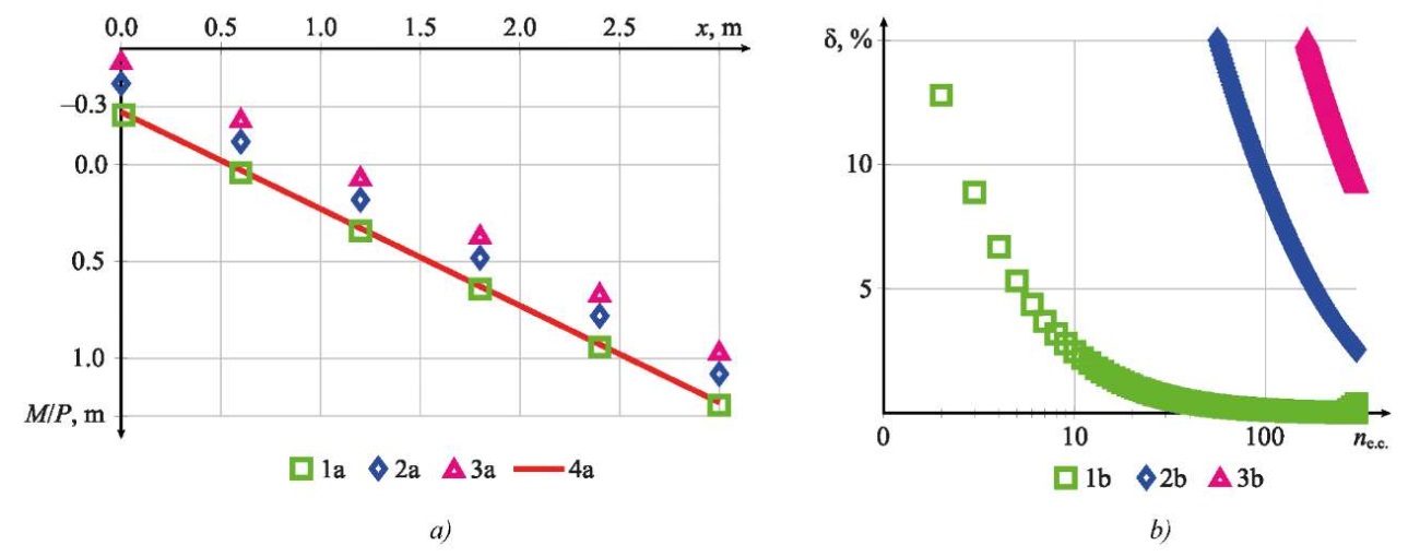
Fig. 7. Results of moment calculations for example 1:
a — calculation results of bending moment M depending on x;
b — calculation error depending on the number of finite elements;
1 a, 1 b — linear approximation and exact stiffness matrix (27);
2 a, 2 b — linear approximation and approximate stiffness matrix (11);
3 a, 3 b — discrete approximation;
4 a — analytical calculation results
Example 2. Example 1, considered previously, represents a case close to the limit, since the stiffness at the left edge of the beam tends to zero. For a more objective assessment of the accuracy of the approaches under consideration, a similar series of calculations was performed for the case of a smooth change in stiffness. Figures 8 and 9 present the results for option 2 of the stiffness change, namely for s0 = 0.6 and s1 = 0.2. The graph of the stiffness function for this option is shown in Figure 5 b.
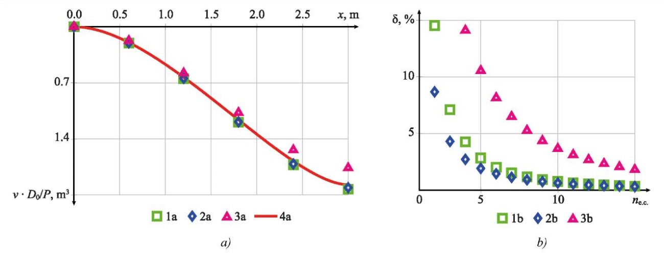
Fig. 8. Results of deflection calculations for example 2:
a —calculation results of deflections v depending on x;
b — calculation error depending on the number of finite elements.
1 a, 1 b — linear approximation and exact stiffness matrix (27);
2 a, 2 b — linear approximation and approximate stiffness matrix (11);
3 a, 3 b — discrete approximation;
4 a — analytical calculation results
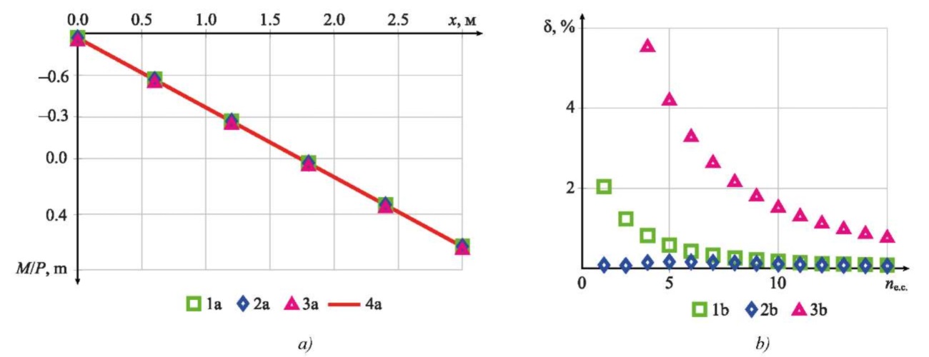
Fig. 9. Results of calculating moments for example 2:
a — calculation results of bending moments M depending on x;
b — calculation error depending on the number of finite elements.
1 a, 1 b — linear approximation and exact stiffness matrix (27);
2 a, 2 b — linear approximation and approximate stiffness matrix (11);
3 a, 3 b — discrete approximation;
4 a — analytical calculation results
Example 3. The problem of bending of a clamped beam under a distributed load. The sketch is shown in Figure 4 b. The calculation results in Figures 10 and 11 were obtained for option 1 of the stiffness distribution, i.e., for s0 = 0.001 and s1 = 1.
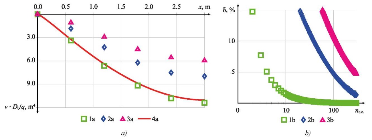
Fig. 10. Results of deflection calculations for example 3:
a — calculation results of deflections v depending on x;
b — calculation error depending on the number of finite elements;
1 a, 1 b — inear approximation and exact stiffness matrix (27);
2 a, 2 b — linear approximation and approximate stiffness matrix (11);
3 a, 3 b — discrete approximation;
4 a — analytical calculation results
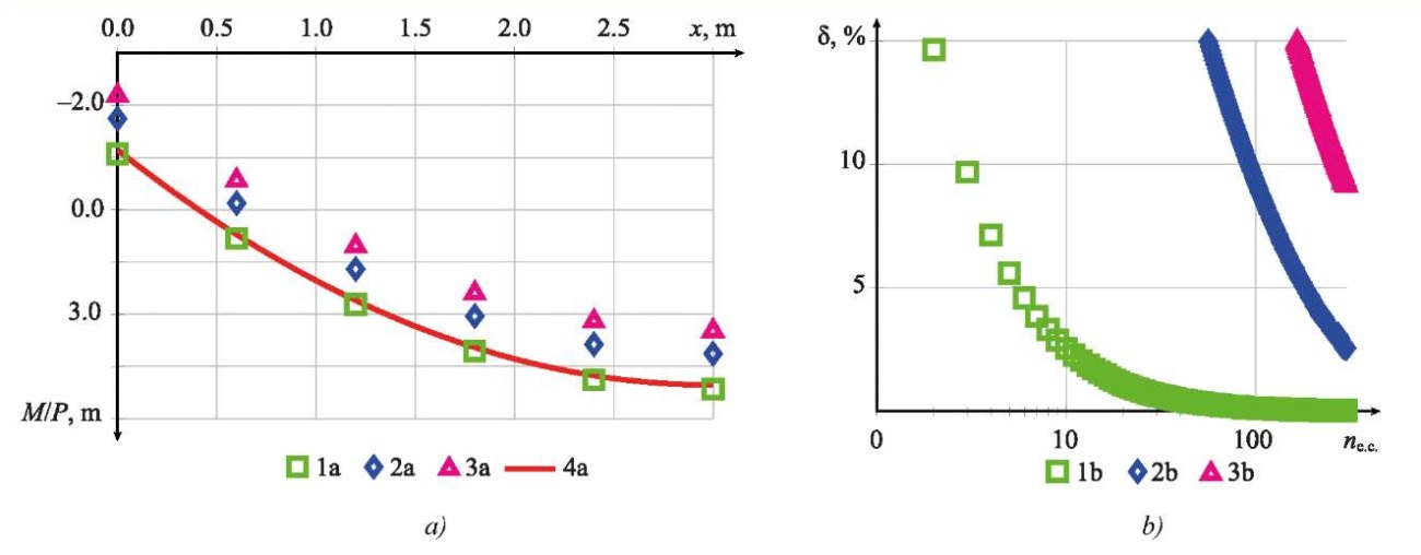
Fig. 11. Results of calculating moments for example 3:
a — calculation results of bending moments M depending on x;
b — calculation error depending on the number of finite elements;
1 a, 1 b — linear approximation and exact stiffness matrix (27);
2 a, 2 b — linear approximation and approximate stiffness matrix (11);
3 a, 3 b — discrete approximation;
4 a — analytical calculation results
Discussion. Based on the analysis of the results shown in Figures 6 and 7, the following conclusions were formulated. In cases of significant changes in stiffness, as in Example 1, only the exact stiffness matrix (27) provided obtaining results comparable with an analytical calculation. In this case, the threshold accuracy of 5% was attained with five finite elements for displacements (Fig. 6 b) and with six finite elements (Fig. 7 b) for bending moments. Using the approximate stiffness matrix (11), similar accuracy was attained only with 90 and 180 finite elements for deflections and moments, respectively. Discrete approximation allowed us to obtain the threshold accuracy for deflections with 220 finite elements. For moments, the required accuracy for discrete approximation was not attained even with 400 elements.
The calculation results for a distributed load, shown in Figures 10 and 11 for Example 3, are similar to those shown in Figures 6 and 7 for Example 1. The key difference is that the accuracy of the results when using the approximate matrix (11) and the discrete approximation has decreased. Thus, it can be concluded that the calculation results are affected not only by the stiffness matrix — exact or approximate — but also by the vector of nodal forces from distributed loads.
Based on the calculation results for a smooth change in stiffness, shown in Figures 8 and 9 for Example 2, the following conclusions were drawn. The approximate (11) and exact (27) finite element stiffness matrices for a smooth change in beam stiffness along its length allowed for comparable results with fewer elements. For example, to attain an error of 5% when calculating deflections using the proposed matrices, no more than four finite elements were required, compared with eight for discrete approximation. Thus, even in the case of a smooth change in stiffness, a linear approximation within a finite element allowed for a two-fold reduction in the degree of discretization of the calculation model, while maintaining comparable calculation accuracy.
The results presented in Figure 8 b and Figure 9 b have a unique feature. The results obtained by the approximate stiffness matrix (11) with the same number of elements showed a smaller deviation from the analytical solution than the results obtained by the exact matrix (27). This was due to the convexity (Fig. 5) of the stiffness change function along the length. In this case, the area of the figure bounded above by the approximation was smaller than the initial. Consequently, the deflection value obtained by the linear approximation was greater (0 а). From the results of calculating the coefficients of the approximate (11) and exact matrix (27), shown in Figure 3, it was clear that the approximate matrix (11) had greater stiffness, which partially compensated for this effect and reduced the total error. Below is matrix [ΔK], whose coefficients were calculated from the formula where  где
где  — coefficients of matrix (11);
  — coefficients of matrix (27). The calculations were performed for parameters ψ0 = 0.664, ψ1 = 0.2, D0 = 1.0 and L = 0.6, which corresponds to the fifth finite element for option 2 of the stiffness distribution.
 (38)
(38)
The average value of the coefficients of matrix (38) is 1.098. Therefore, the stiffness of finite element 5 will be approximately 10% higher if the approximate stiffness matrix is used (11).
Conclusion. This paper proposes and verifies an approach to constructing stiffness matrices for beam finite elements with linear stiffness change along their length. Both approximate (based on a variational solution to the problem) and exact (by analytical integration of a differential equation) stiffness matrices and corresponding nodal load vectors are obtained. The key advantages of the resulting matrices are the following.
Linear stiffness approximation provides an optimal balance between accuracy, complexity, and computational resources, making the proposed method a practical tool for analyzing real-world structures with variable stiffness. A comparison of calculation results using an approximate and exact stiffness matrix shows that the approximate matrix allows for attaining the required accuracy with high precision and lower computational costs for beams with smoothly varying stiffness along their length. For rapid changes in stiffness along the length, as well as in extreme cases, to obtain significantly higher accuracy while maintaining the same number of elements, it is recommended to use the exact (27) stiffness matrix. Discrete approximation is only applicable in cases of smooth changes in stiffness along the length.
The resulting stiffness matrices open up possibilities for more accurate and efficient analysis of real structures, including reinforced concrete elements, taking into account physical nonlinearity — this determines the direction of further research. It is also planned to obtain a geometric stiffness matrix for solving stability problems and a mass matrix for dynamic analysis.
1. Chepurnenko AS, Turina VS, Akopyan VF. Optimization of Rectangular and Box Sections in Oblique Bending and Eccentric Compression. Construction Materials and Products. 2023;6(5):1–14. https://doi.org10.58224/2618-7183-2023-6-5-2
2. Sventikov AA, Kuznetsov DN. Strength and Deformability of Steel Beams with a Step-by-Step Change in Wall Thickness. Russian Journal of Building Construction and Architecture. 2025;1(77):14–23. https://doi.org/10.36622/2541-7592.2025.77.1.002
3. Godínez-Domínguez E, Tena-Colunga A, Velázquez-Gutiérrez I, Silvestre-Pascacio R. Parametric Study of the Bending Stiffness of RC Cracked Building Beams. Engineering Structures. 2021;243:112695. https://doi.org/10.1016/j.engstruct.2021.112695
4. Abuizeih YQY, Tamov MM, Leonova AN, Mailyan DR, Nikora NI. Numerical Simulation of Nonlinear Bending Behaviour of UHPC Beams. Construction Materials and Products. 2025;8(4):6. https://doi.org/10.58224/2618-7183-2025-8-4-6
5. Jun Zhao, Yibo Jiang, Gaochuang Cai, Xiangsheng Deng, Amir Si Larbi. Flexural Stiffness of RC Beams with High-Strength Steel Bars after Exposure to Elevated Temperatures. Structural Concrete. 2024;25(5):3081–3102. https://doi.org/10.1002/suco.202300934
6. Imamović D, Skrinar M. Static Bending Analysis of a Transversely Cracked Strip Tapered Footing on a Two-Parameter Soil Using a New Beam Finite Element. Continuum Mechanics and Thermodynamics. 2024;36:571– 584. https://doi.org/10.1007/s00161-024-01283-7
7. Volkov AV, Golubkin KS. Analysis of Shear Stress Distribution in a Rod with Tapered Cross-Section in Gradient Elasticity Theory. Mechanics of Composite Materials and Structures. 2025;31(1):40–56. https://doi.org/10.33113/mkmk.ras.2025.31.01.04
8. Rao Hota VS Ganga, Spyrakos CC. Closed Form Series Solutions of Boundary Value Problems with Variable Properties. Computers & Structures. 1986;23(2):211–215. https://doi.org/10.1016/0045-7949(86)90213-0
9. Banerjee JR, Williams FW. Exact Bernoulli–Euler Static Stiffness Matrix for a Range of Tapered Beams. International Journal for Numerical Methods in Engineering. 1986;23(9):1707–1719. https://doi.org/10.1002/nme.1620230904
10. Yagofarov AKh. Calculation of a Two-Span Uncut Beam of Variable Rigidity with Equal Spans. News of Higher Educational Institutions. Construction. 2021;(754(10)):55–65. https://doi.org/10.32683/0536-1052-2021-754-10-55-65
11. Karamysheva AA, Yazyeva SB, Chepurnenko AS. Calculation of Plane Bending Stability of Beams with Variable Stiffness. Bulletin of Higher Educational Institutions. North Caucasus region. Technical Sciences. 2016;(186(1)):95–98. https://doi.org/10.17213/0321-2653-2016-1-95-98
12. Just DJ. Plane Frameworks of Tapering Box and I-Section. Journal of the Structural Division. 1977;103(1):71–86. https://doi.org/10.1061/jsdeag.0004549
13. Brown CJ. Approximate Stiffness Matrix for Tapered Beams. Journal of Structural Engineering (ASCE). 1984;110(12):3050–3055. https://doi.org/10.1061/(ASCE)0733-9445(1984)110:12(3050)
14. Cherednichenko AP, Potelzheko EA, Tyufanov VA. Methods for Calculating Beams with Variable Stiffness. In: Proc. International Student Construction Forum-2017. Vol. 1. Belgorod: Belgorod State Technological University named after V.G. Shukhov; 2017. P. 249–252.
15. Ziou H, Guenfoud M. Simple Incremental Approach for Analysing Optimal Non-Prismatic Functionally Graded Beams. Advances in Civil and Architectural Engineering. 2023;14(26):118–137. https://doi.org/10.13167/2023.26.8
16. Bui Thi Thu Hoai, Le Cong Ich, Nguyen Dinh Kien. Size-Dependent Nonlinear Bending of Tapered Cantilever Microbeam Based on Modified Couple Stress Theory. Vietnam Journal of Science and Technology. 2024;62(6):1196–1209. https://doi.org/10.15625/2525-2518/19281
17. Haskul M, Kisa M. Free Vibration of the Double Tapered Cracked Beam. Inverse Problems in Science and Engineering. 2021;29(11):1537–1564. https://doi.org/10.1080/17415977.2020.1870971
18. Hosseinian N, Attarnejad R. A Novel Finite Element for the Vibration Analysis of Tapered Laminated Plates. Polymer Composites. 2024;45(10):8732–8743. https://doi.org/10.1002/pc.28372
19. Nesterov VA. Stiffness Matrix of the Tridimensional Beam Finite Element with Low Transverse Shear Stiffness. Siberian Aerospace Journal. 2010;29(3):71–75.
20. Gaidzhurov PP, Saveleva NA. Application of the Double Approximation Method for Constructing Stiffness Matrices of Volumetric Finite Elements. Advanced Engineering Research (Rostov-on-Don). 2023;23(4):365–375. https://doi.org/10.23947/2687-1653-2023-23-4-365-375
21. Zeinali Y, Jamali M, Musician S. General Form of the Stiffness Matrix of a Tapered Beam-column. International Journal of Mining, Metallurgy & Mechanical Engineering (IJMMME). 2013;1(3):149–153.
22. Peng He, Zhansheng Liu, Chun Li. An Improved Beam Element for Beams with Variable Axial Parameters. Shock and Vibration. 2013;20(4):601–617. https://doi.org/10.3233/SAV-130771
23. Ceba AI. Stiffness Matrix for Bars with Variable Section or Inertia. International Journal of Materials Science and Applications. 2025;14(1):13–28. https://doi.org/10.11648/j.ijmsa.20251401.12
24. Rezaiee-Pajand M, Masoodi AR, Bambaeechee MT. Tapered Beam–Column Analysis by Analytical Solution. Proceedings of the Institution of Civil Engineers — Structures and Buildings. 2019;172(11):789–804. https://doi.org/10.1680/jstbu.18.00062
25. Li Xia Meng, Nian Li Lu, Shi Ming Liu. Exact Expression of Element Stiffness Matrix for a Tapered Beam and Its Application in Stability Analysis. Advanced Materials Research. 2011;255–260:1968–1973. https://doi.org/10.4028/www.scientific.net/AMR.255-260.1968
26. Fedorinin NI, Solomonov KN, Tishchuk LI. Universal Equation of Elastic Line of a Beam of Linear Rigidity. News of Tula State University. Technical Sciences. 2022;(9):517–521. https://doi.org/10.24412/2071-6168-2022-9-517-521
27. Ksenofontova TK, Mareeva OV, Verkhoglyadova AS. Calculation of Monolithic Buildings Structures Taking into Account the Nonlinear Operation of Reinforced Concrete. Construction Materials and Products. 2024;7(1):1–8. https://doi.org/10.58224/2618-7183-2024-7-1-4
28. Deryugin EE. Simplified Calculation of the Inertia Moment of the Cross Section of the Console under Loading. Advanced Engineering Research (Rostov-on-Don). 2024;24(2):159–169. https://doi.org/10.23947/2687-1653-2024-24-2-159-169.
Nikita Yu. Tsybin, Cand.Sci. (Eng.), Associate Professor of the Department of Strength of Materials
26, Yaroslavskoye Shosse, Moscow, 129337
ResearcherID: I-3045-2016
Scopus Author ID: 56966570000
A new approach for calculating beams with variable stiffness along their length is developed. Exact and approximate stiffness matrices for beam finite elements are obtained. Improved calculation accuracy and reduced required model discretization are demonstrated. Criteria for choosing between exact and approximate element stiffness matrices are presented. The results are suitable for integration into structural analysis software packages. The method can be applied to the analysis of reinforced concrete beams, as well as beam stability and dynamics.
Tsybin N.Yu. Exact and Approximate Stiffness Matrix and Nodal Load Vector for a Beam Finite Element with Linearly Varying Stiffness along Its Length. Advanced Engineering Research (Rostov-on-Don). 2025;25(4):275-289. https://doi.org/10.23947/2687-1653-2025-25-4-2206. EDN: VHVNIF


Advanced Engineering Research (Rostov-on-Don)
ISSN 2687-1653 (Online)
Contact with: Publisher / Editorial Office of the Journal
Publisher: Don State Technical University - DSTU, Rostov-on-Don, Russia - https://donstu.ru/en/
Editor-in-Chief: Alexey N. Beskopylny, Dr.Sci. (Eng.), Professor, Vice-Rector, Don State Technical University (Rostov-on-Don, Russia)
Don State Technical University
1, Gagarin Sq., Rostov-on-Don, 344003, Russia
tel.: +7 (863) 2738-372, e-mail: vestnik@donstu.ru
16+
Processing of personal data